Unsupervised Clustering
Bruno Grande
2017-06-26
Hierarchical Clustering
We plot the expression of the 1000 most variably expressed genes before and after correction as heatmaps below to verify that batch effects have indeed been corrected.
Original Expression Values
heatmap_clean_vst_most_var  <-
  plot_heatmap(most_var(salmon$clean$vst, ntop), colours)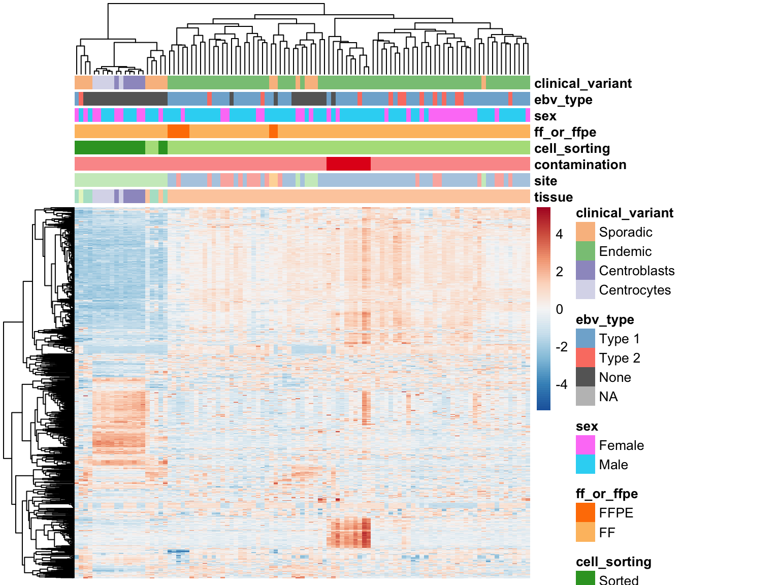
Corrected Expression Values
heatmap_clean_cvst_most_var <-
  plot_heatmap(most_var(salmon$clean$cvst, ntop), colours)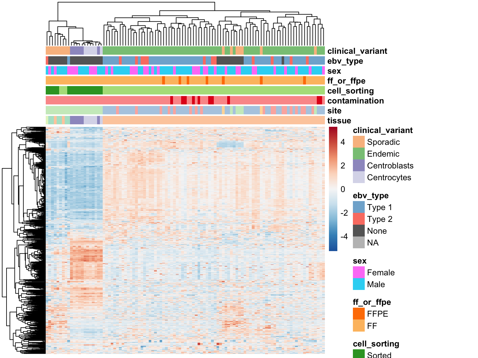
EBV Gene Expression
ebv_genes_idx <- rownames(salmon$clean$cvst) %in% ebv_genes

heatmap_salmon_no_mz_ebv <-
  salmon$clean$cvst[ebv_genes_idx,] %>%
  plot_heatmap(colours, scale = "none", cutree_cols = 2,
               clustering_distance_cols = "euclidean")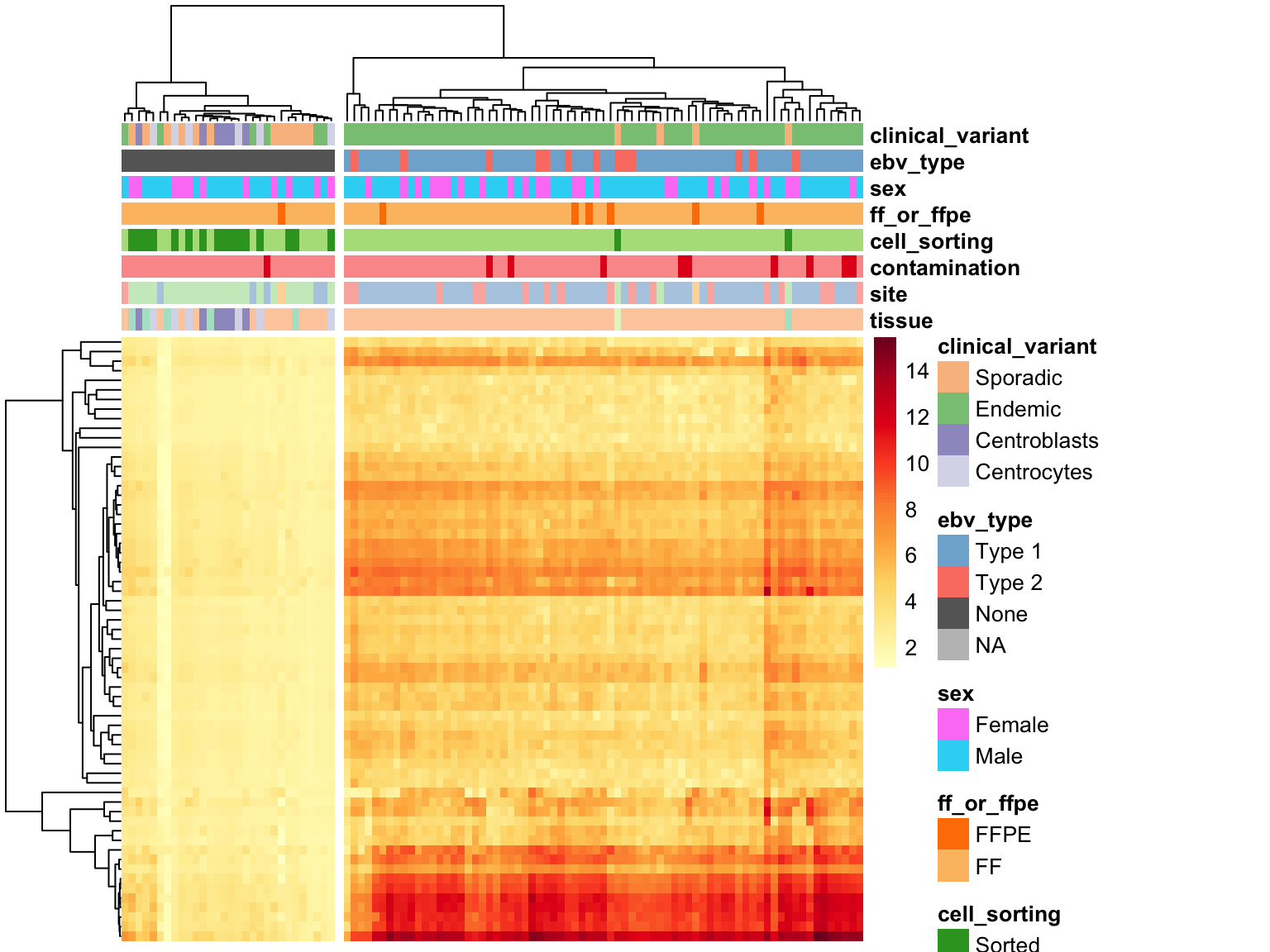
measured_genes  <- rownames(salmon$raw$counts)
ebvpos_patients <- rownames(annotations)[annotations$ebv_type != "None"]
latency_annot   <-
  latency_genes %>%
  mutate_at(vars(-gene), function(x) ifelse(x == 0, "Absent", "Present")) %>%
  as.data.frame() %>%
  column_to_rownames("gene")
latency_colours <-
  names(latency_annot) %>%
  set_names() %>%
  map(~ c(Absent = "#bfbfbf", Present = "#666666"))

latency_genes %>%
  filter(gene %in% measured_genes) %$%
  salmon$raw$counts[gene, ebvpos_patients] %>%
  {log10(1 + .)} %>%
  plot_heatmap(c(colours, latency_colours),
               metadata = annotations[, -grep("lib_date", names(annotations))],
               annotation_row = rev(latency_annot), scale = "none",
               cluster_rows = FALSE, clustering_distance_cols = "correlation")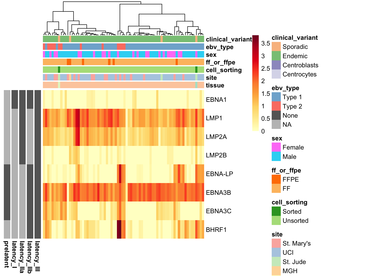
Sample Correlations
salmon$clean$cor <- cor(assay(salmon$clean$cvst))

corplot_salmon_clean <- plot_heatmap(
  salmon$clean$cor, colours, colData(salmon$clean$dds), scale = "none",
  treeheight_row = 0)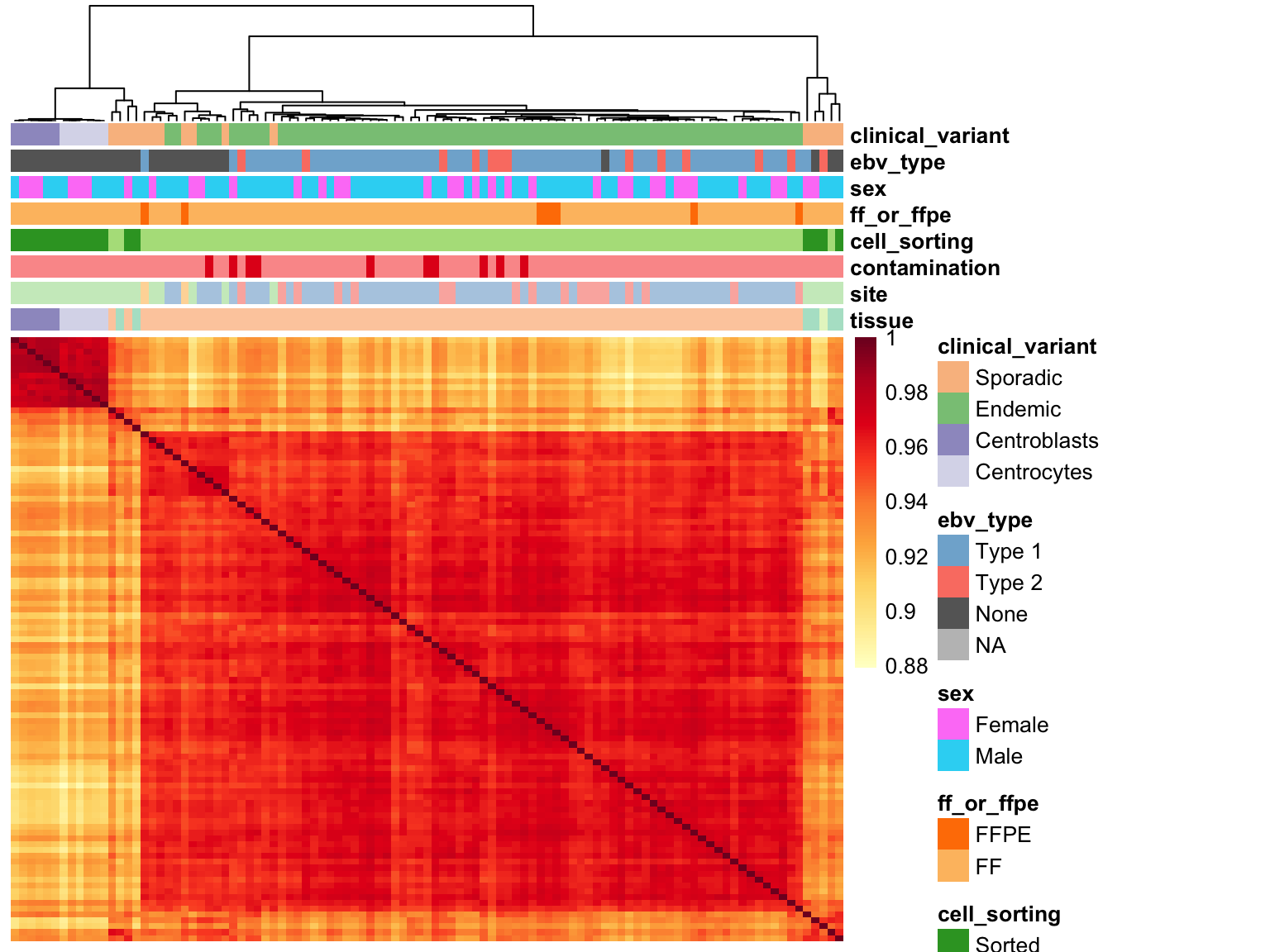
Principal Component Analysis
salmon$clean$pca <- calc_pca(salmon$clean$cvst)

pca_salmon_clean_plots <-
  names(colData(salmon$clean$dds)) %>%
  stringr::str_subset("^(?!SV)") %>%
  map(~plot_pca(salmon$clean$pca, .x, colours, c(1,1)))

screeplot_salmon <-
  salmon$clean$pca$percent_var %>%
  slice(1:10) %>%
  ggplot(aes(x = pc, y = percent_var, group = "all")) +
  geom_point() +
  geom_line() +
  labs(title = "PCA Scree Plot")

pca_salmon_clean_plots <- c(pca_salmon_clean_plots, list(screeplot_salmon))

gridExtra::grid.arrange(grobs = pca_salmon_clean_plots, ncol = 3)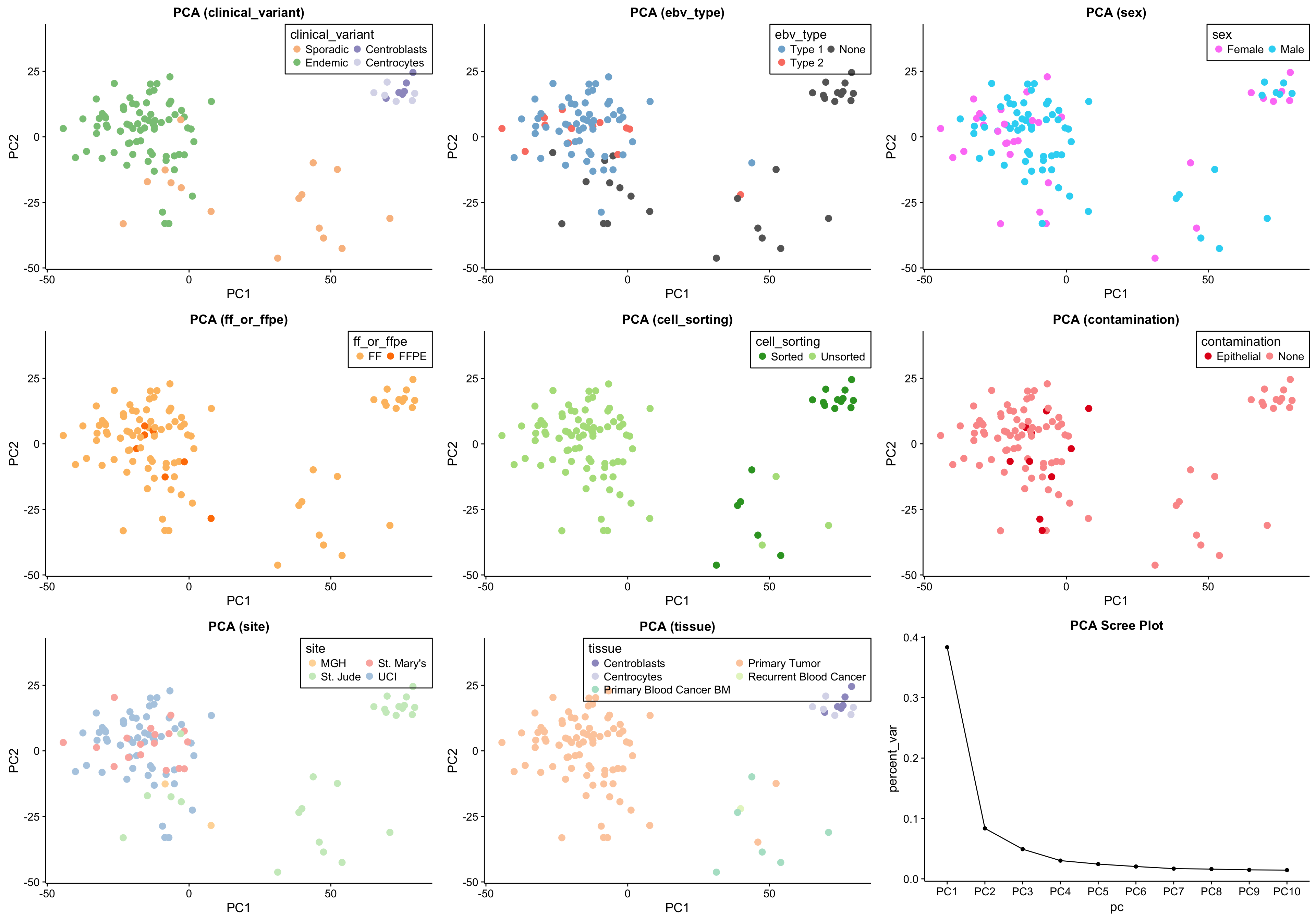
DLBCL Classifiers
mBL signature genes
heatmap_salmon_clean_mbl <-
  plot_heatmap(salmon$clean$cvst[genes$mbl, ], colours)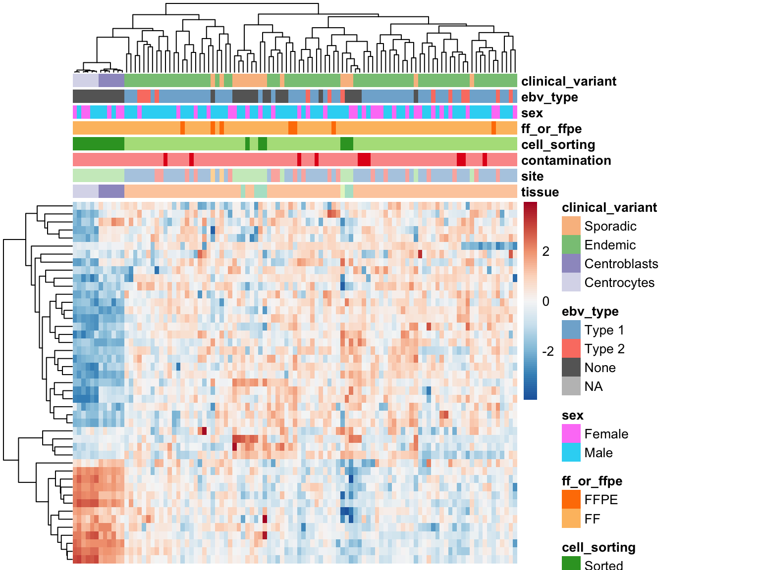
Morgan BL-DLBCL classifier
heatmap_salmon_clean_morgan <-
  plot_heatmap(salmon$clean$cvst[genes$morgan, ], colours)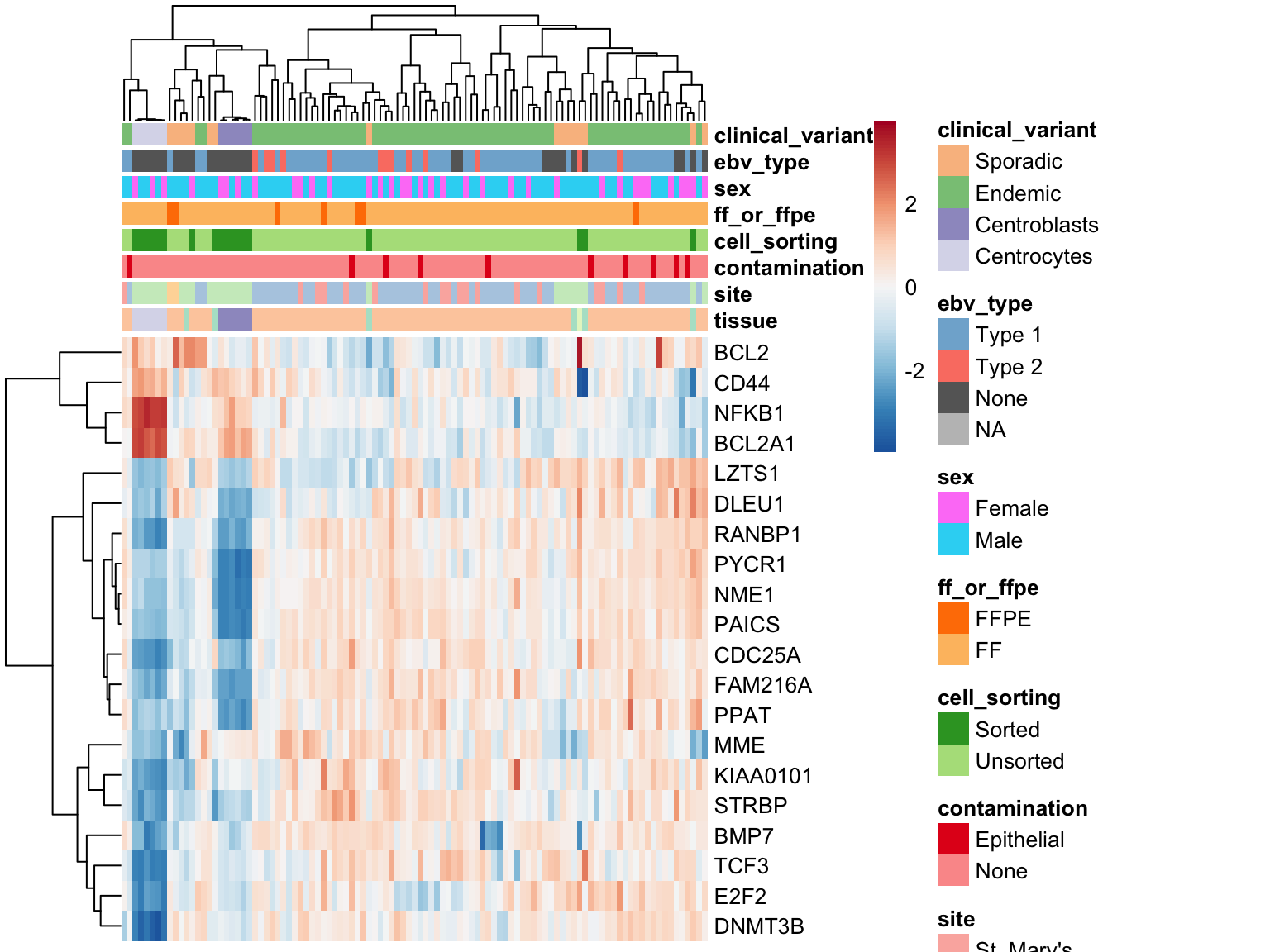
Wright COO classifier
heatmap_salmon_clean_wright <-
    plot_heatmap(salmon$clean$cvst[genes$wright, ], colours, border_color = NA)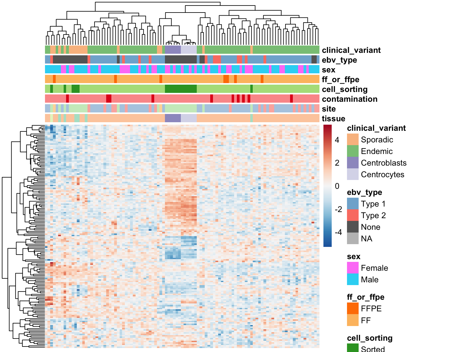
Special Gene Lists
heatmap_salmon_clean_malaria <-
    plot_heatmap(salmon$clean$cvst[genes$malaria, ], colours, border_color = NA)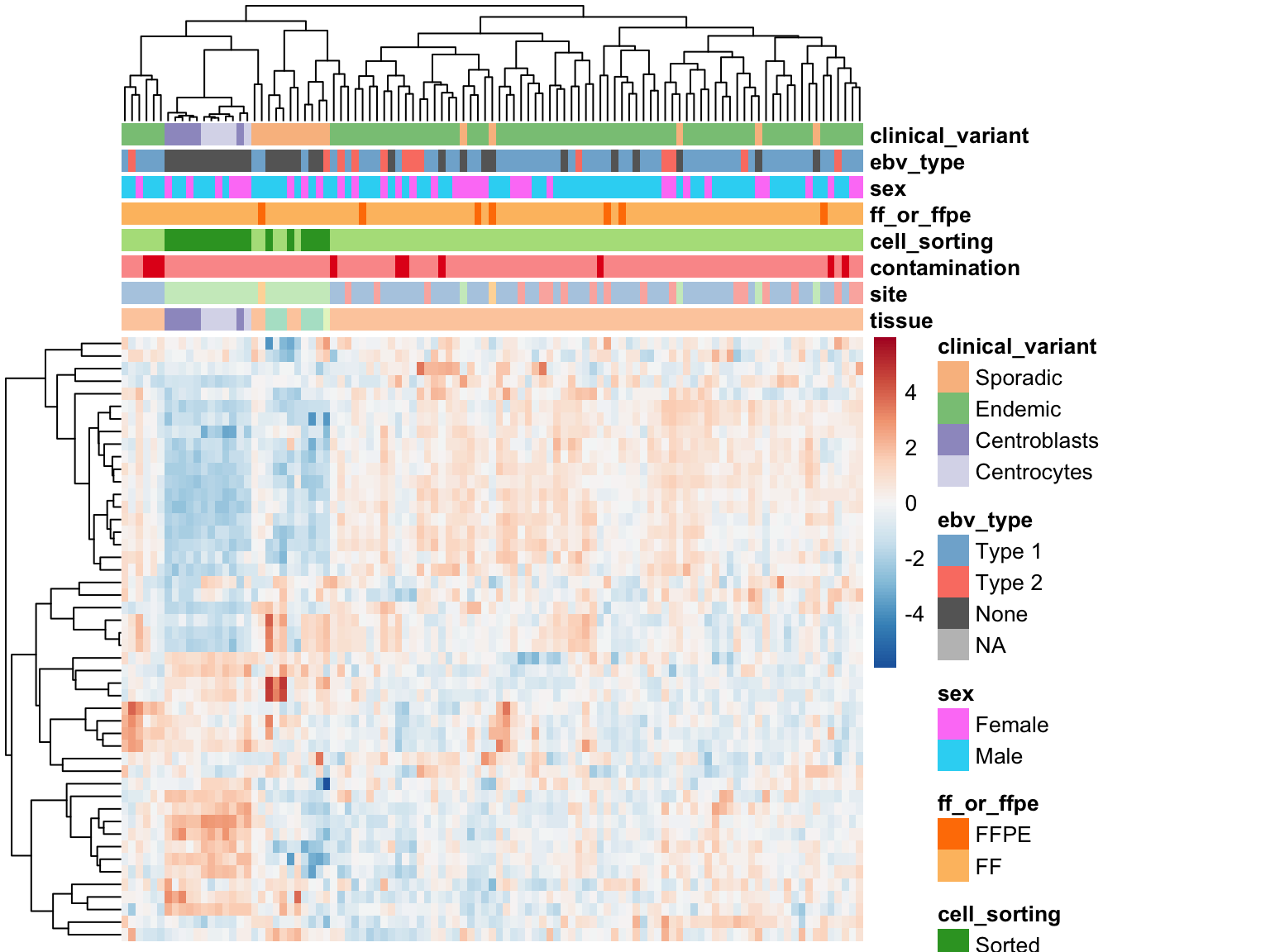
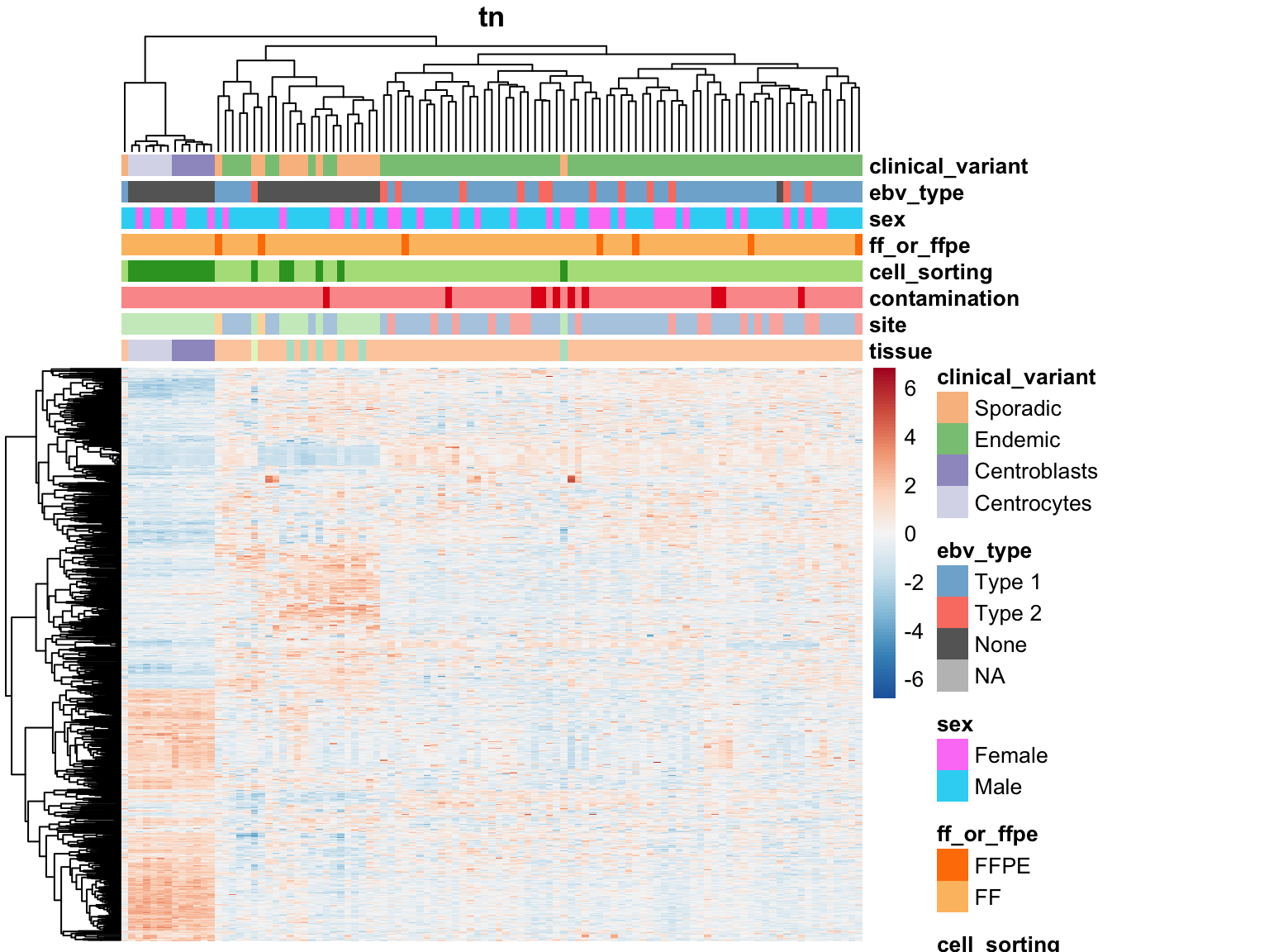
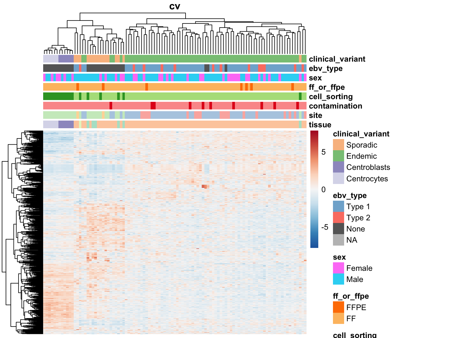
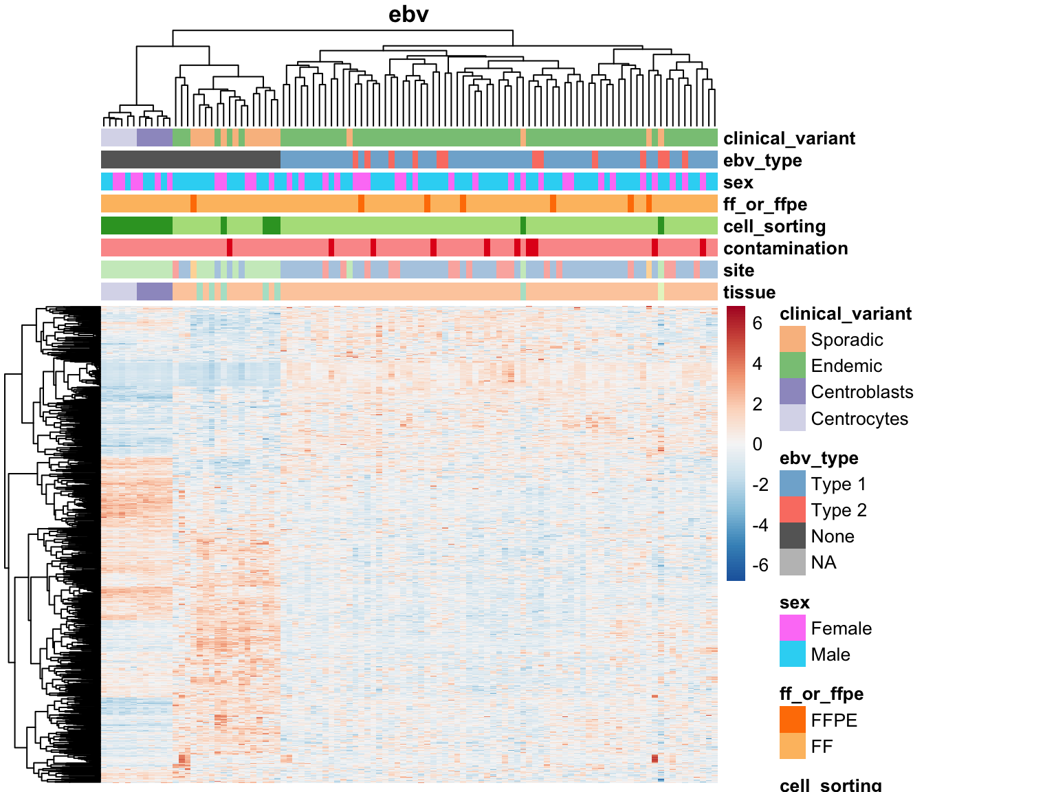
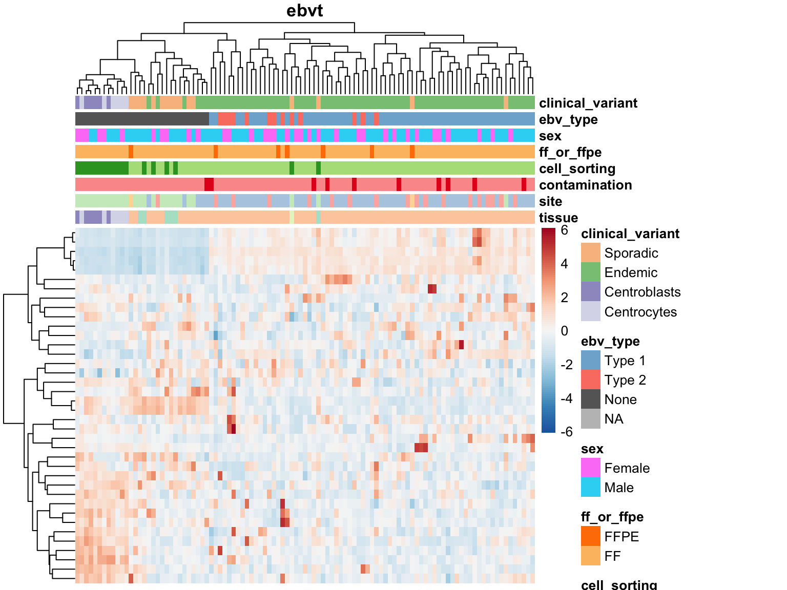
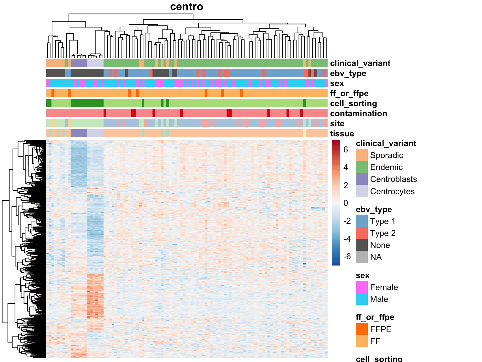
Differentially Expressed Genes
Tumour Metadata
for (var in names(salmon$clean$de)) {
  plot_heatmap(salmon$clean$cvst[get_sig_genes(salmon$clean$de[[var]]$lfc_0),] %>% most_var(1000),
               colours, main = var)
}
Mutations
for (var in names(salmon$muts$de)) {
  plot_heatmap(salmon$clean$cvst[get_sig_genes(salmon$muts$de[[var]]$lfc_0),] %>% most_var(1000),
               colours, main = var)
}