barplot_maf_mutfreq_data <-
maf@data %>%
dplyr::count(patient, ff_or_ffpe, Variant_Type) %>%
dplyr::ungroup() %>%
tidyr::spread(Variant_Type, n) %>%
dplyr::mutate(patient = forcats::fct_reorder(patient, -SNP)) %>%
tidyr::gather(Variant_Type, n, -patient, -ff_or_ffpe) %>%
dplyr::mutate(
Variant_Type = dplyr::recode_factor(
Variant_Type, SNP = "SNV", INS = "Insertion", DEL = "Deletion"),
Variant_Class = dplyr::recode_factor(
Variant_Type, SNV = "SNVs", Insertion = "Indels", Deletion = "Indels"),
cohort = ifelse(grepl("^BL", patient), "BLGSP", "ICGC"))
barplot_maf_mutfreq_stats <-
barplot_maf_mutfreq_data %>%
dplyr::group_by(Variant_Class, patient) %>%
dplyr::summarise(n = sum(n)) %>%
dplyr::summarise(n_patients = dplyr::n_distinct(patient),
max = max(n),
mean = round(mean(n)))
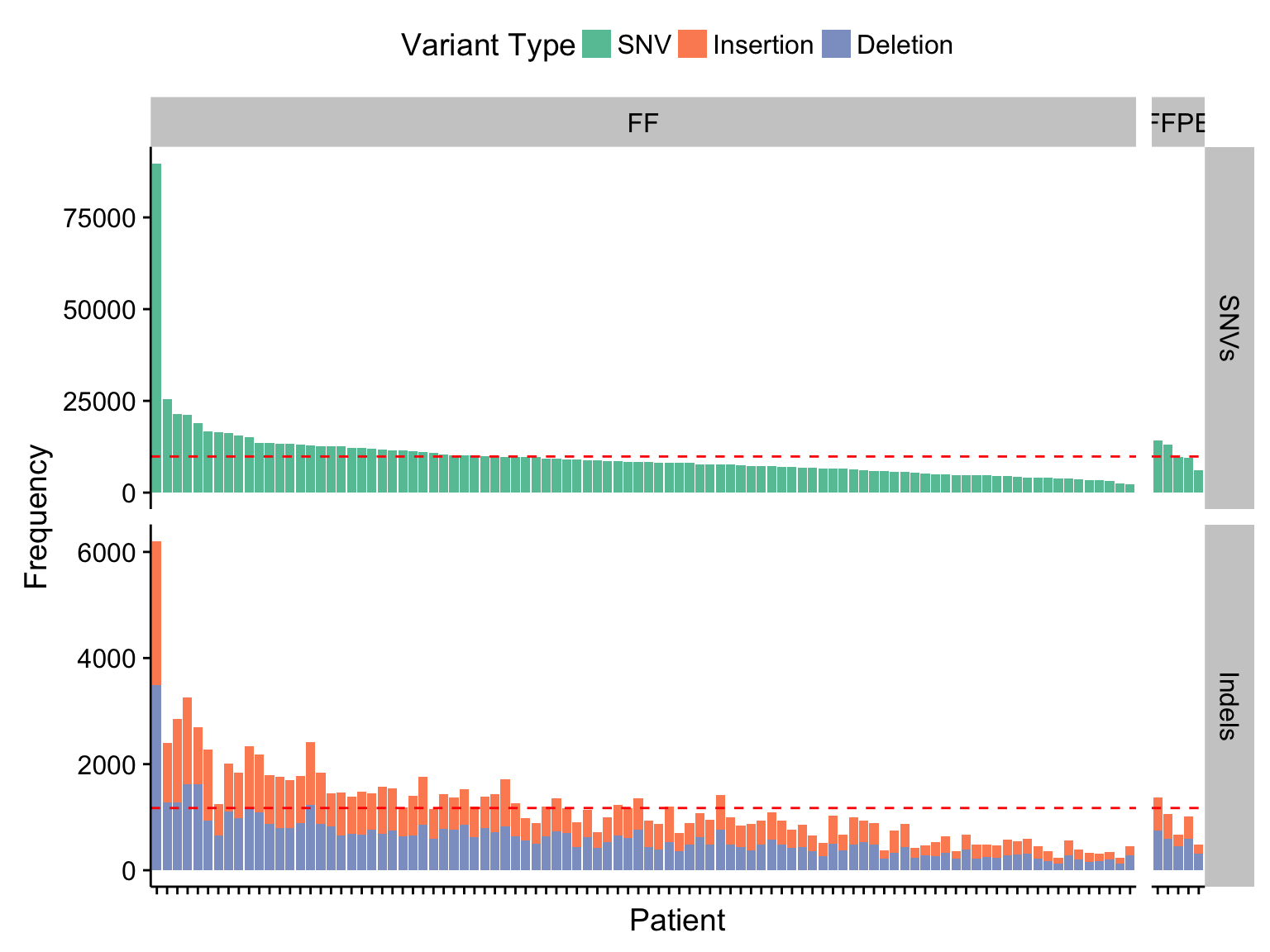
barplot_maf_mutfreq_ff_or_ffpe <-
ggplot(barplot_maf_mutfreq_data) +
geom_col(aes(x = patient, y = n, fill = Variant_Type)) +
geom_hline(data = barplot_maf_mutfreq_stats, aes(yintercept = mean),
colour = "red", linetype = 2) +
facet_grid(Variant_Class ~ ff_or_ffpe, scales = "free", space = "free_x") +
scale_x_discrete(labels = NULL) +
scale_fill_brewer(palette = "Set2") +
theme(legend.position = "top") +
rotate_x_text() +
labs(x = "Patient", y = "Frequency", fill = "Variant Type")
barplot_maf_mutfreq_ff_or_ffpe
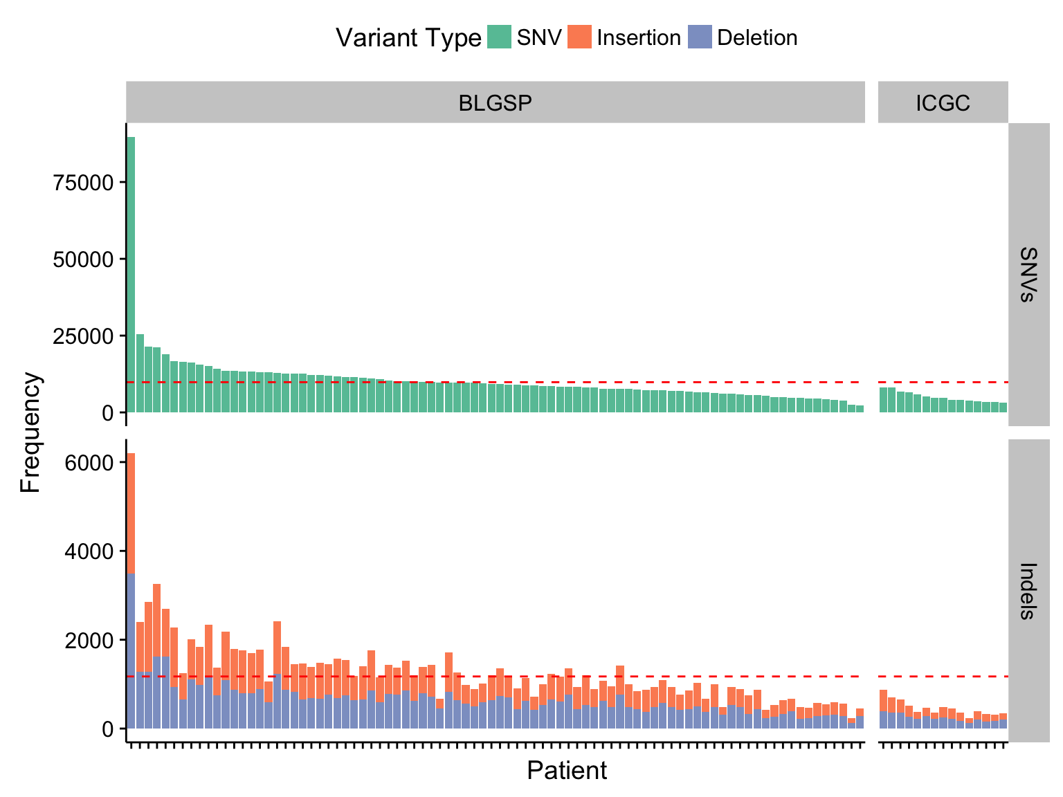
barplot_maf_mutfreq_cohort <-
  barplot_maf_mutfreq_ff_or_ffpe +
  facet_grid(Variant_Class ~ cohort, scales = "free", space = "free_x")

barplot_maf_mutfreq_cohort
maf_mutfreq_age <-
metadata$patient %>%
select(patient, age = age_at_initial_pathologic_diagnosis, ebv_type, clinical_variant) %>%
inner_join(barplot_maf_mutfreq_data, by = "patient") %>%
drop_na() %>%
filter(
Variant_Class == "SNVs",
patient != "BL142",
age < 20,
n < 50000)
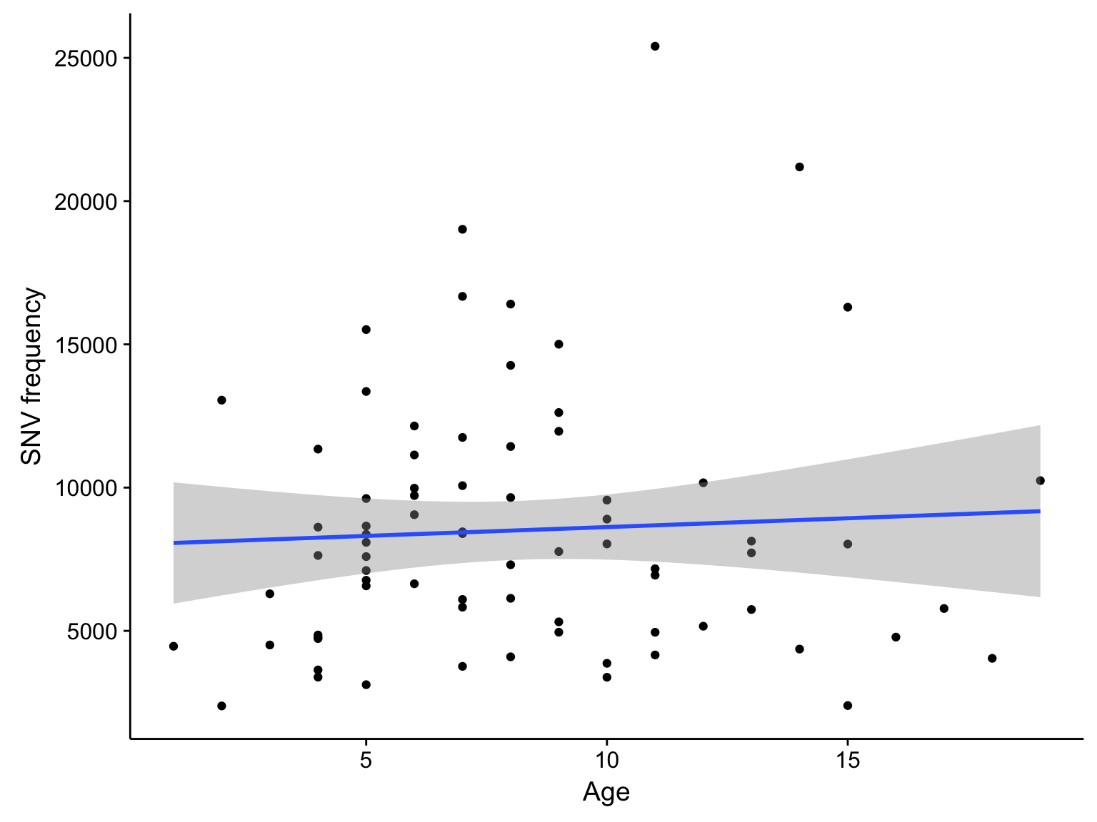
scatterplot_maf_mutfreq_age <-
maf_mutfreq_age %>%
ggplot(aes(age, n)) +
geom_point() +
geom_smooth(method = "lm") +
labs(x = "Age", y = "SNV frequency")
scatterplot_maf_mutfreq_age
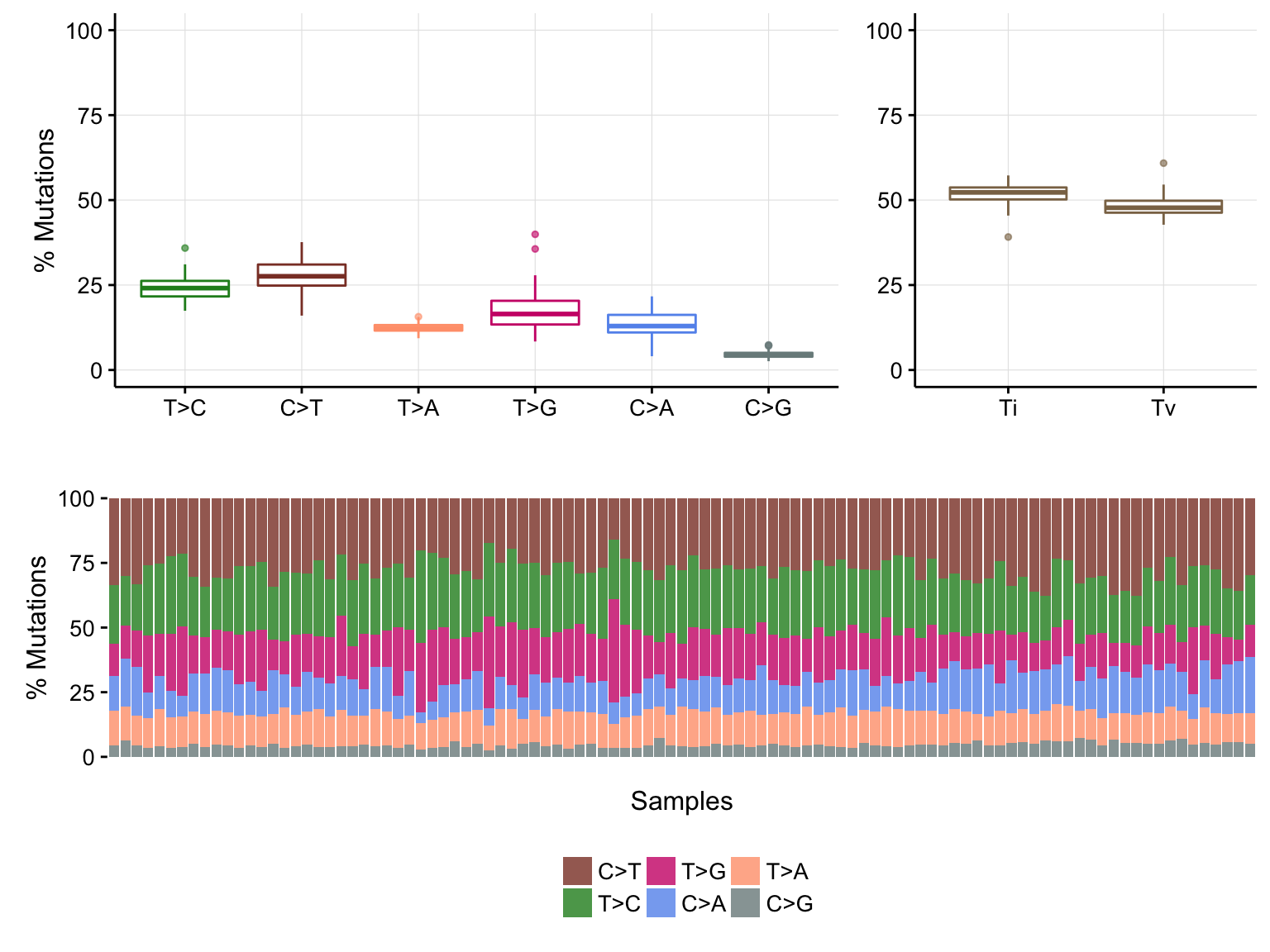
maf_titv <- titv(maf, useSyn = TRUE, plot = FALSE)

plotTiTv(maf_titv)
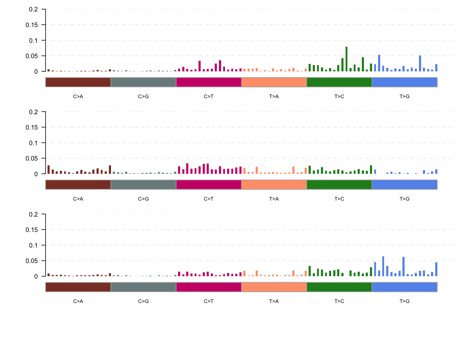
maf_tnm <- trinucleotideMatrix(maf, paths$genome_grch37, useSyn = TRUE)
maf_sig <- extractSignatures(maf_tnm, nTry = 6, plotBestFitRes = FALSE)
   method   seed rng metric rank sparseness.basis sparseness.coef      rss      evar
1: brunet random   3     KL    2        0.3029940       0.3938290 18005848 0.9513736
2: brunet random   5     KL    3        0.3498756       0.3776821  5358215 0.9855297
3: brunet random   4     KL    4        0.3803052       0.3181127  3448177 0.9906879
4: brunet random   2     KL    5        0.3890917       0.2558792  2991051 0.9919224
5: brunet random   1     KL    6        0.4013064       0.2792355  2541249 0.9931371
   silhouette.coef silhouette.basis residuals niter   cpu cpu.all nrun cophenetic dispersion
1:       1.0000000        1.0000000  25270.52   510 0.208  15.686   10  0.9950794  0.9498402
2:       0.8275758        0.7747530  18418.03  1060 0.386  15.708   10  0.9819025  0.8571356
3:       0.7297531        0.7486916  13965.73   780 0.238  16.756   10  0.9761288  0.8512303
4:       0.5195405        0.6024173  12421.42   880 0.353  19.530   10  0.9420168  0.7367003
5:       0.3865825        0.5544854  11294.23  1970 0.823  18.969   10  0.9326400  0.7234075
   silhouette.consensus
1:            0.9790992
2:            0.9059049
3:            0.9029230
4:            0.7321543
5:            0.6582883
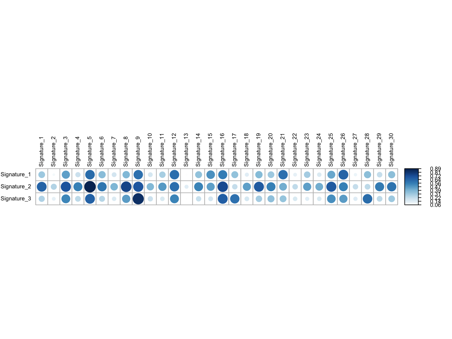
corrplot::corrplot(maf_sig$coSineSimMat, is.corr = FALSE, tl.cex = 0.6,
                   tl.col = 'black', cl.cex = 0.6)
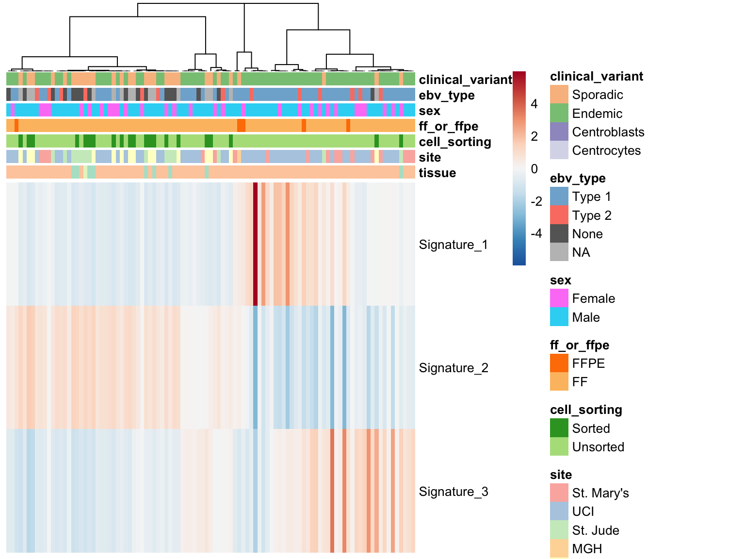
maf_sig$contributions %>%
  set_colnames(get_patient_id(colnames(.))) %>%
  plot_heatmap(colours, gannotations, cluster_rows = FALSE)
mut_counts <- maf@data[Variant_Type == "SNP",
.(N = .N, ebv_status),
by = "Tumor_Sample_Barcode"] %>%
distinct()
maf_signatures_mut_burden <-
maf_sig$contributions %>%
t() %>%
as.data.frame() %>%
rownames_to_column("Tumor_Sample_Barcode") %>%
as.data.table() %>%
merge(mut_counts, by = "Tumor_Sample_Barcode") %>%
gather(signature, value, starts_with("Sig"))
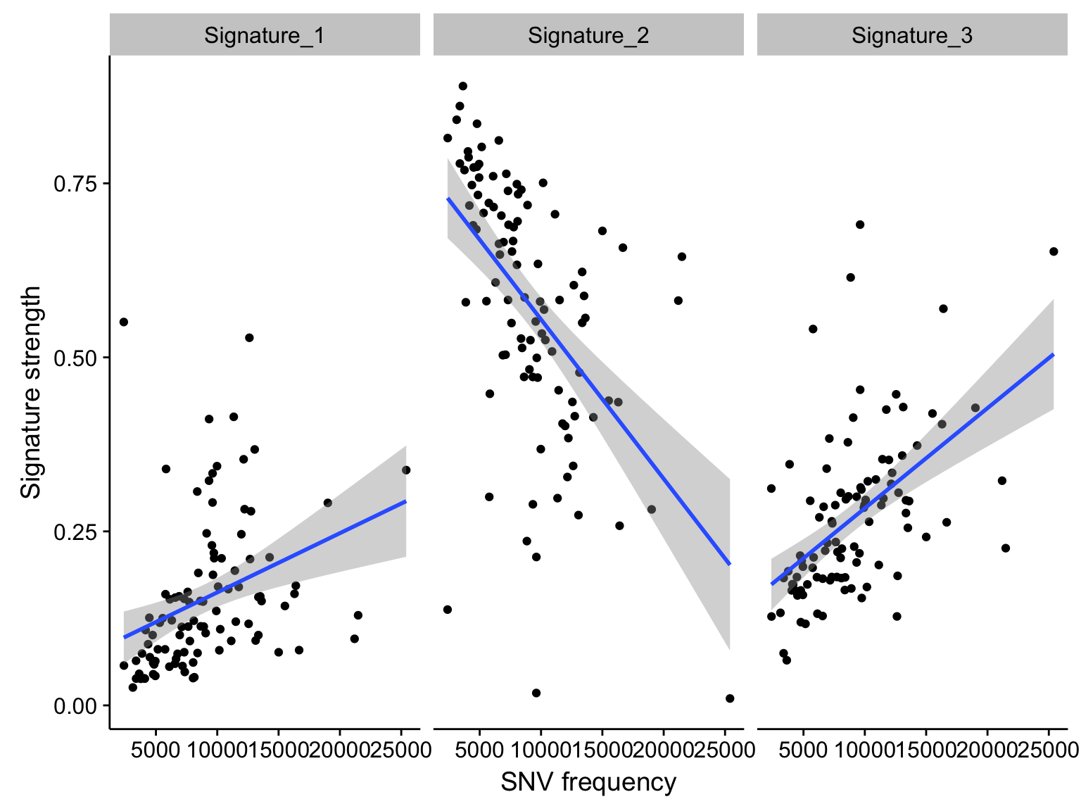
scatterplot_maf_signatures_mut_burden <-
maf_signatures_mut_burden %>%
filter(N < 50000) %>%
ggplot(aes(N, value)) +
geom_point() +
geom_smooth(method = "lm") +
facet_grid(~ signature) +
labs(x = "SNV frequency", y = "Signature strength")
scatterplot_maf_signatures_mut_burden
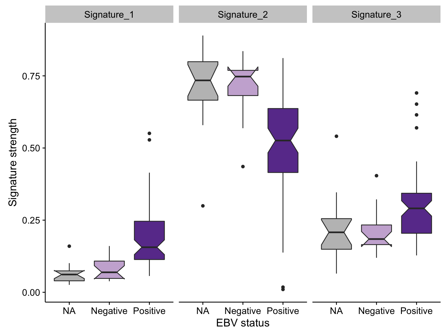
boxplot_maf_signatures_ebv <-
  maf_signatures_mut_burden %>%
  filter(N < 50000) %>%
  ggplot(aes(ebv_status, value, fill = ebv_status)) +
  geom_boxplot(notch = TRUE) +
  facet_grid(~ signature) +
  scale_fill_manual(values = colours$ebv_status, breaks = NULL) +
  labs(x = "EBV status", y = "Signature strength")

boxplot_maf_signatures_ebv
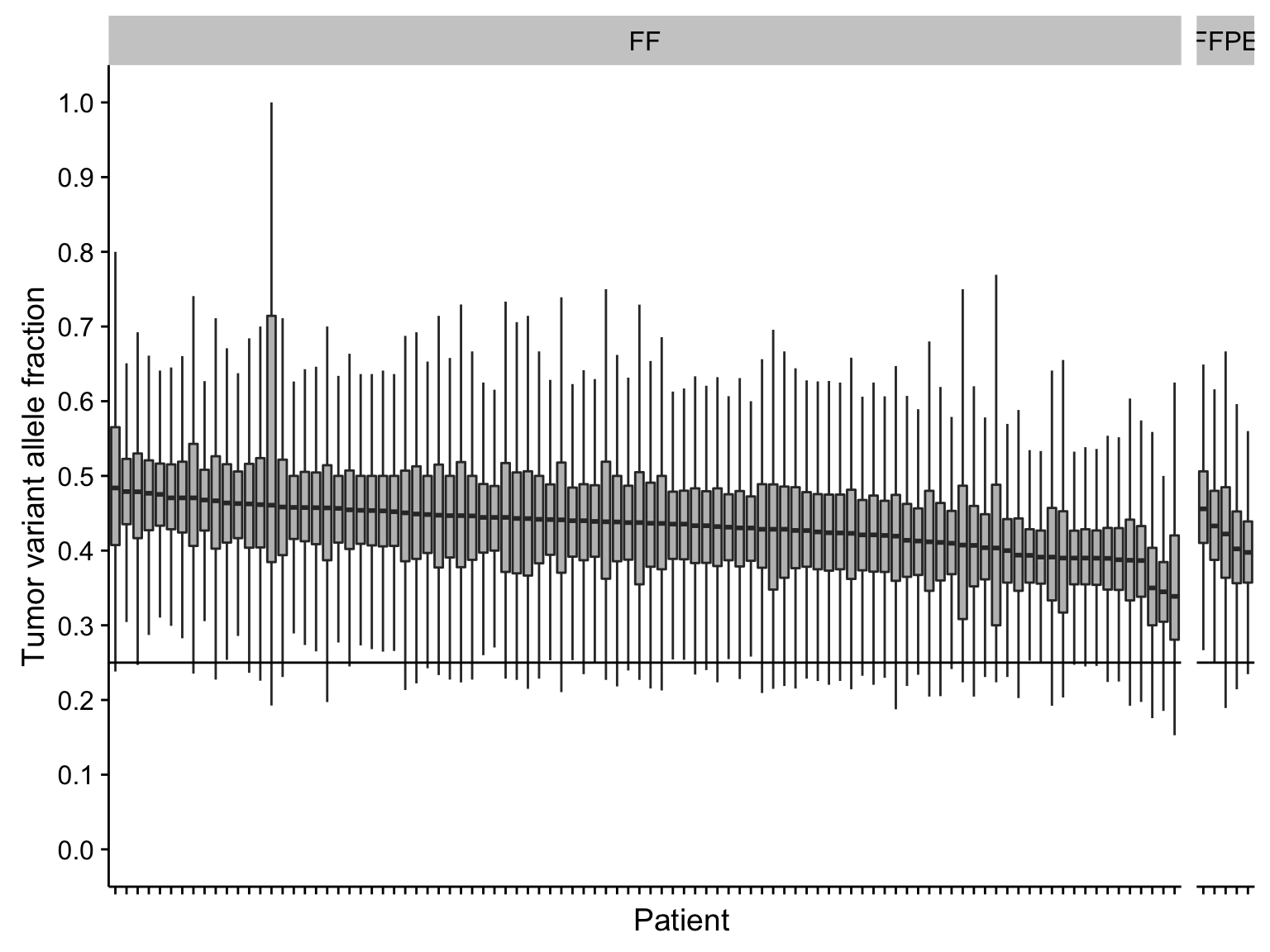
boxplot_maf_vaf <-
  maf@data %>%
  mutate(
    patient = fct_reorder(patient, t_vaf, function(x) -median(x)),
    is_bl_gene = Hugo_Symbol %in% genes$bl & is_nonsynonymous(Consequence)) %>%
  ggplot(aes(patient, t_vaf)) +
  geom_boxplot(fill = "grey", outlier.colour = NA) +
  geom_hline(yintercept = c(0.25)) +
  scale_x_discrete(labels = NULL) +
  scale_y_continuous(breaks = seq(0, 1, 0.1), limits = c(0, 1)) +
  facet_grid(~ff_or_ffpe, scales = "free_x", space = "free_x") +
  rotate_x_text() +
  labs(x = "Patient", y = "Tumor variant allele fraction")

boxplot_maf_vaf
nonsyn_query <- "Variant_Classification %in% c('Missense', 'Truncation', 'Splicing', 'Multi_Hit')"
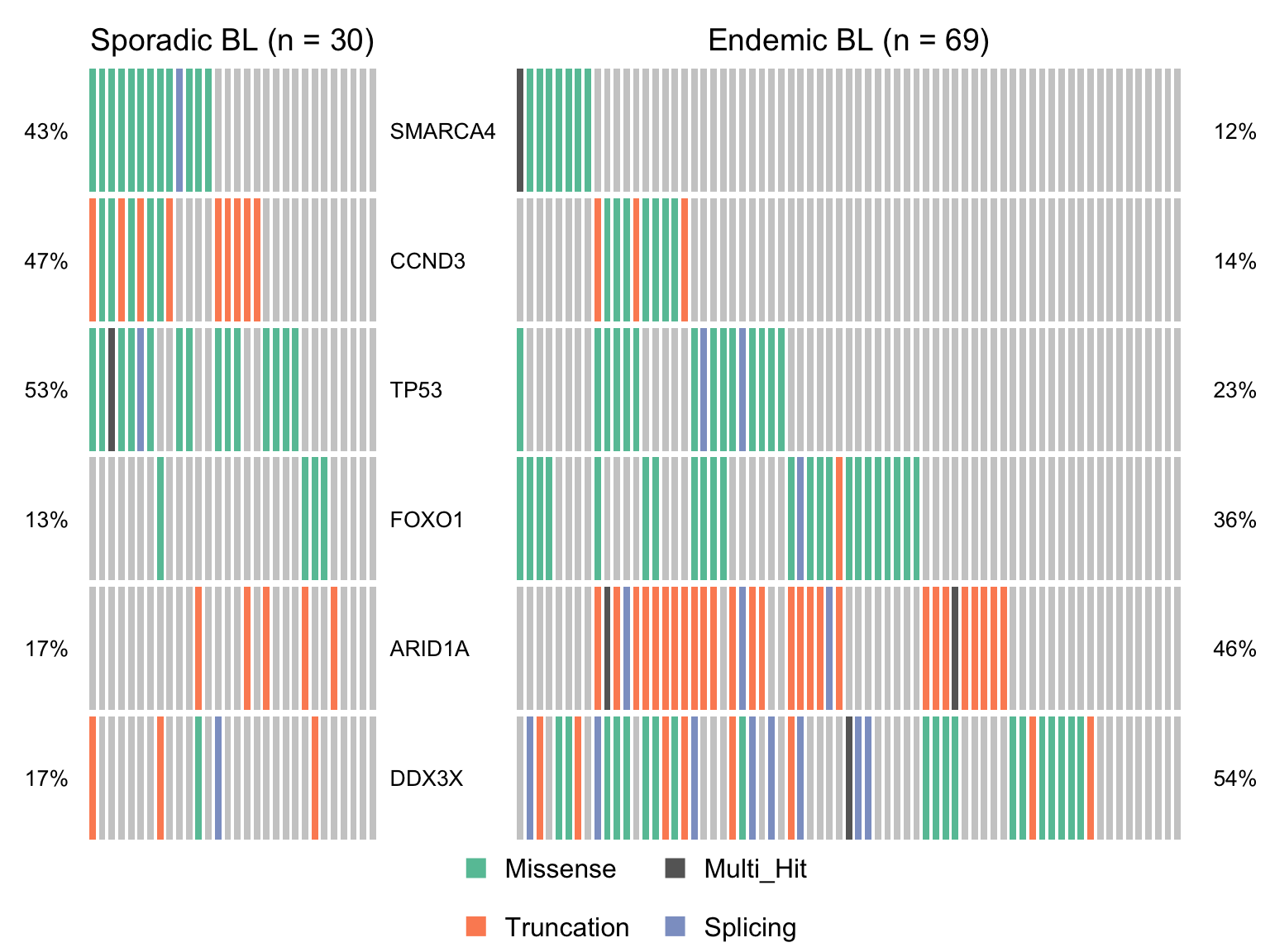
maf_ebl <- subsetMaf(maf, query = paste("clinical_variant == 'Endemic' &", nonsyn_query),
includeSyn = TRUE, mafObj = TRUE, genes = smgs)
maf_sbl <- subsetMaf(maf, query = paste("clinical_variant == 'Sporadic' &", nonsyn_query),
includeSyn = TRUE, mafObj = TRUE, genes = smgs)
maf_ebl_vs_sbl <- mafCompare(maf_ebl, maf_sbl, 'Endemic BL', 'Sporadic BL', minMut = 4)
sig_genes_ebv_vs_sbl <-
maf_ebl_vs_sbl$results %>%
filter(Hugo_Symbol %in% smgs) %$%
Hugo_Symbol[pval < 0.05][order(or[pval < 0.05])]
if (length(sig_genes_ebv_vs_sbl) > 0) {
cooncoplot_maf_ebl_vs_sbl <- coOncoplot(
maf_sbl, maf_ebl, sig_genes_ebv_vs_sbl,
m1Name = 'Sporadic BL', m2Name = 'Endemic BL',
removeNonMutated = FALSE, colors = colours$categs)
# print(cooncoplot_maf_ebl_vs_sbl)
}
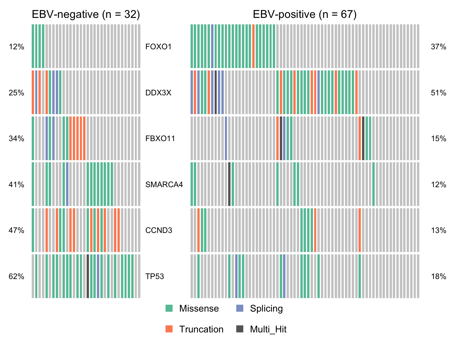
maf_ebvneg <- subsetMaf(maf, query = paste("ebv_status == 'Negative' &", nonsyn_query),
                         includeSyn = TRUE, mafObj = TRUE, genes = smgs)
maf_ebvpos <- subsetMaf(maf, query = paste("ebv_status == 'Positive' &", nonsyn_query),
                        includeSyn = TRUE, mafObj = TRUE, genes = smgs)

maf_ebvneg_vs_ebvpos <- mafCompare(maf_ebvneg, maf_ebvpos,
                                   'EBV-negative', 'EBV-positive', minMut = 4)

sig_genes_ebvneg_vs_ebvpos <-
  maf_ebvneg_vs_ebvpos$results %>%
  filter(Hugo_Symbol %in% smgs) %$%
  Hugo_Symbol[pval < 0.05][order(or[pval < 0.05])]

if (length(sig_genes_ebvneg_vs_ebvpos) > 0) {
  cooncoplot_maf_ebvneg_vs_ebvpos <- coOncoplot(
    maf_ebvneg, maf_ebvpos, sig_genes_ebvneg_vs_ebvpos,
    m1Name = 'EBV-negative', m2Name = 'EBV-positive',
    removeNonMutated = FALSE, colors = colours$categs)

  # print(cooncoplot_maf_ebvneg_vs_ebvpos)
}
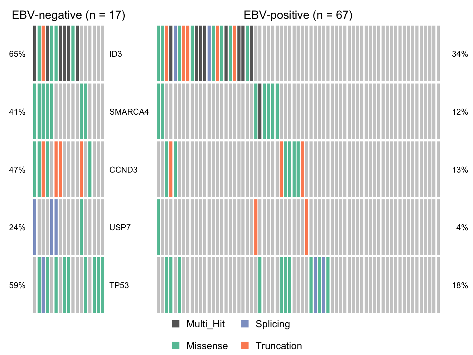
maf_ebvneg <- subsetMaf(maf, query = paste("ebv_status %in% c('Negative', 'NA') &", nonsyn_query),
                         includeSyn = TRUE, mafObj = TRUE, genes = smgs)
maf_ebvpos <- subsetMaf(maf, query = paste("ebv_status == 'Positive' &", nonsyn_query),
                        includeSyn = TRUE, mafObj = TRUE, genes = smgs)

maf_ebvneg_vs_ebvpos <- mafCompare(maf_ebvneg, maf_ebvpos,
                                   'EBV-negative', 'EBV-positive', minMut = 4)

sig_genes_ebvneg_vs_ebvpos <-
  maf_ebvneg_vs_ebvpos$results %>%
  filter(Hugo_Symbol %in% smgs) %$%
  Hugo_Symbol[pval < 0.05][order(or[pval < 0.05])]

if (length(sig_genes_ebvneg_vs_ebvpos) > 0) {
  cooncoplot_maf_ebvneg_vs_ebvpos <- coOncoplot(
    maf_ebvneg, maf_ebvpos, sig_genes_ebvneg_vs_ebvpos,
    m1Name = 'EBV-negative', m2Name = 'EBV-positive',
    removeNonMutated = FALSE, colors = colours$categs)

  # print(cooncoplot_maf_ebvneg_vs_ebvpos)
}
maf_ebv1 <- subsetMaf(maf, query = paste("ebv_type == 'Type 1' &", nonsyn_query),
                         includeSyn = TRUE, mafObj = TRUE, genes = smgs)
maf_ebv2 <- subsetMaf(maf, query = paste("ebv_type == 'Type 2' &", nonsyn_query),
                        includeSyn = TRUE, mafObj = TRUE, genes = smgs)


maf_ebv1_vs_ebv2 <- mafCompare(maf_ebv1, maf_ebv2,
                               'EBV Type 1', 'EBV Type 2', minMut = 4)

sig_genes_ebv1_vs_ebv2 <-
  maf_ebv1_vs_ebv2$results %>%
  filter(Hugo_Symbol %in% smgs) %$%
  Hugo_Symbol[pval < 0.05][order(or[pval < 0.05])]

if (length(sig_genes_ebv1_vs_ebv2) > 0) {
  cooncoplot_maf_ebv1_vs_ebv2 <- coOncoplot(
    maf_ebv1, maf_ebv2, c(sig_genes_ebv1_vs_ebv2, "TP53"),
    m1Name = 'EBV Type 1', m2Name = 'EBV Type 2',
    removeNonMutated = FALSE, colors = colours$categs)

  # print(cooncoplot_maf_ebv1_vs_ebv2)
}
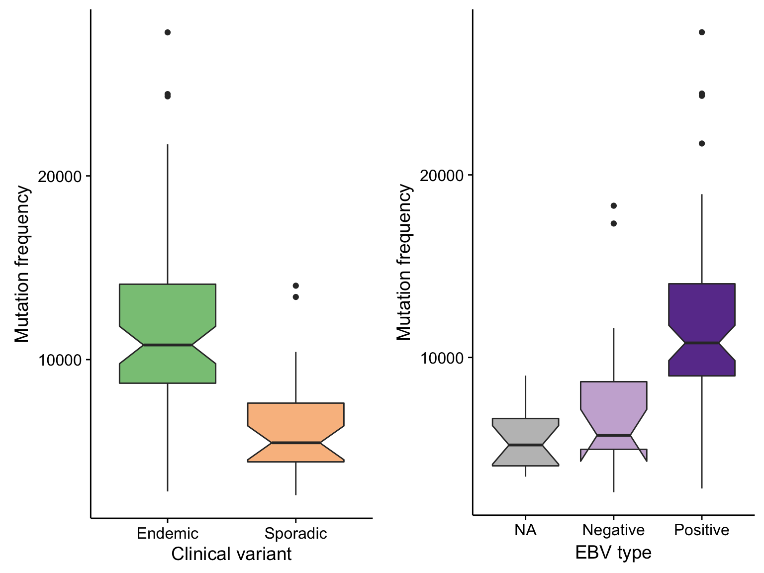
boxplot_maf_compare_all_mutfreq_cv <-
  maf@data %>%
  count(clinical_variant, Tumor_Sample_Barcode) %>%
  filter(n < 50000) %>%
  ggplot(aes(clinical_variant, n, fill = clinical_variant)) +
  geom_boxplot(notch = TRUE) +
  scale_fill_manual(values = colours$clinical_variant, breaks = NULL) +
  labs(x = "Clinical variant", y = "Mutation frequency")

boxplot_maf_compare_all_mutfreq_ebv <-
  maf@data %>%
  count(ebv_status, Tumor_Sample_Barcode) %>%
  filter(n < 50000) %>%
  ggplot(aes(ebv_status, n, fill = ebv_status)) +
  geom_boxplot(notch = TRUE) +
  scale_fill_manual(values = colours$ebv_status, breaks = NULL) +
  # scale_x_discrete(limits = c("Positive", "Negative")) +
  labs(x = "EBV type", y = "Mutation frequency")

gridExtra::grid.arrange(
  boxplot_maf_compare_all_mutfreq_cv, boxplot_maf_compare_all_mutfreq_ebv, ncol = 2)
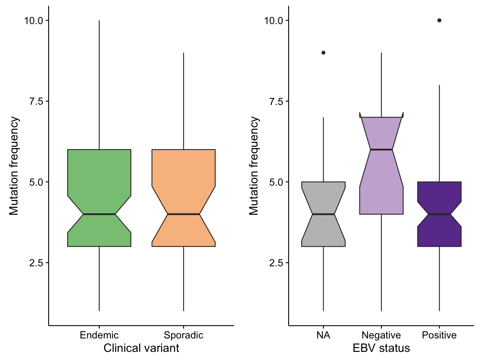
boxplot_maf_compare_nonsyn_smg_mutfreq_cv <-
  maf@data %>%
  filter(is_nonsynonymous(Consequence), Hugo_Symbol %in% smgs) %>%
  count(clinical_variant, Tumor_Sample_Barcode) %>%
  ggplot(aes(clinical_variant, n, fill = clinical_variant)) +
  geom_boxplot(notch = TRUE) +
  scale_fill_manual(values = colours$clinical_variant, breaks = NULL) +
  labs(x = "Clinical variant", y = "Mutation frequency")

boxplot_maf_compare_nonsyn_smg_mutfreq_ebv <-
  maf@data %>%
  filter(is_nonsynonymous(Consequence), Hugo_Symbol %in% smgs) %>%
  count(ebv_status, Tumor_Sample_Barcode) %>%
  ggplot(aes(ebv_status, n, fill = ebv_status)) +
  geom_boxplot(notch = TRUE) +
  scale_fill_manual(values = colours$ebv_status, breaks = NULL) +
  labs(x = "EBV status", y = "Mutation frequency")

gridExtra::grid.arrange(
  boxplot_maf_compare_nonsyn_smg_mutfreq_cv, boxplot_maf_compare_nonsyn_smg_mutfreq_ebv, ncol = 2)
ig_loci <- GRanges(
  c("chr2", "chr8", "chr14", "chr22"),
  IRanges(c(88999518, 128747246, 106020156, 22942470),
          c(89599757, 128753246, 107349540, 23342167)))

chroms    <- c(paste0("chr", 1:22), "chrX")
seqlens   <- seqlengths(BSgenome.Hsapiens.UCSC.hg19::Hsapiens)[chroms]
gen       <- data.frame(chroms, seqlens) %>% set_colnames(c("V1", "V2"))

gaps_gr <-
  read_tsv_quiet(paths$gaps) %>%
  rename(seqnames = `#chrom`, start = chromStart, end = chromEnd) %>%
  makeGRangesFromDataFrame()

bins <-
  tileGenome(seqlens, tilewidth = 5000, cut.last.tile.in.chrom = TRUE) %>%
  subsetByOverlaps(ig_loci, invert = TRUE)

maf_grl <-
  maf@data %>%
  .[, .(biospecimen_id, Chromosome, Start_Position, End_Position,
        HGVSp_Short, Consequence)] %>%
  .[, Chromosome := sub("^", "chr", Chromosome)] %>%
  .[Chromosome %in% chroms] %>%
  as.data.frame() %>%
  filter_nonsyn(inverse = TRUE) %>%
  makeGRangesListFromDataFrame(
    split.field = "biospecimen_id",
    seqnames.field = "Chromosome",
    start.field = "Start_Position",
    end.field = "End_Position")

mut_counts <-
  map(as.list(maf_grl), ~countOverlaps(bins, .x)) %>%
  map(pmin, 1) %>%
  invoke(cbind, .) %>%
  rowSums()

mut_counts_fit <- fitdistrplus::fitdist(
  mut_counts, distr = "binom", start = list(prob = 0.01),
  fix.arg = list(size = length(maf_grl)))

qval_thres <- 1e-9

mut_counts_df <-
  bins %>%
  as.data.frame() %>%
  inset("count", value = mut_counts) %>%
  select(seqnames, start, end, count) %>%
  mutate(
    pval = map_dbl(count, ~ binom.test(.x, n = length(maf_grl),
                                       p = mut_counts_fit$estimate,
                                       alternative = "greater")$p.value),
    qval = p.adjust(pval, "BH"),
    nlog_qval = -log10(qval),
    signif = qval < qval_thres)

closest_genes_idx <-
  mut_counts_df %>%
  filter(signif) %>%
  makeGRangesFromDataFrame() %>%
  GenomicRanges::nearest(genes_gr)

symbol_annotations <-
  genes_gr[closest_genes_idx] %>%
  as.data.frame() %>%
  select(symbol) %>%
  bind_cols(filter(mut_counts_df, signif), .) %>%
  group_by(symbol) %>%
  top_n(1, -qval) %>%
  select(seqnames, start, end, symbol)
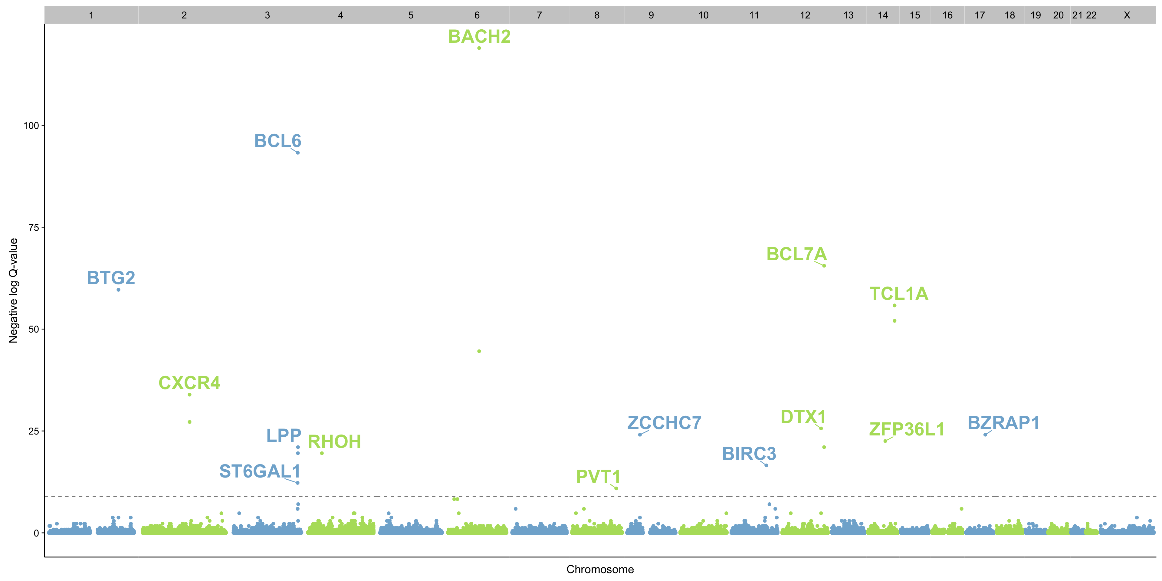
manhattanplot_maf_noncoding_mut_density <-
  mut_counts_df %>%
  left_join(symbol_annotations, by = c("seqnames", "start", "end")) %>%
  mutate(
    seqnames = sub("chr", "", seqnames),
    seqnames = factor(seqnames, levels = c(1:22, "X")),
    colour = ifelse(as.integer(seqnames) %% 2, "even", "odd")) %>%
  filter(nlog_qval > 0) %>%
  ggplot(aes(start, nlog_qval, label = symbol, colour = colour)) +
  geom_point() +
  ggrepel::geom_text_repel(nudge_y = 3, fontface = "bold", size = 8) +
  geom_hline(yintercept = -log10(qval_thres), linetype = 2, colour = "grey40") +
  scale_x_continuous(labels = NULL) +
  scale_colour_manual(values = c(even = "#80b1d3", odd = "#b3de69"), breaks = NULL) +
  facet_grid(~seqnames, scales = "free_x", space = "free_x") +
  theme(
    panel.spacing = unit(0, "lines"),
    axis.ticks.x = element_blank()) +
  labs(x = "Chromosome", y = "Negative log Q-value")

gt <- ggplot_gtable(ggplot_build(manhattanplot_maf_noncoding_mut_density))
gt$layout$clip[grep("panel", gt$layout$name)] <- "off"
grid::grid.draw(gt)
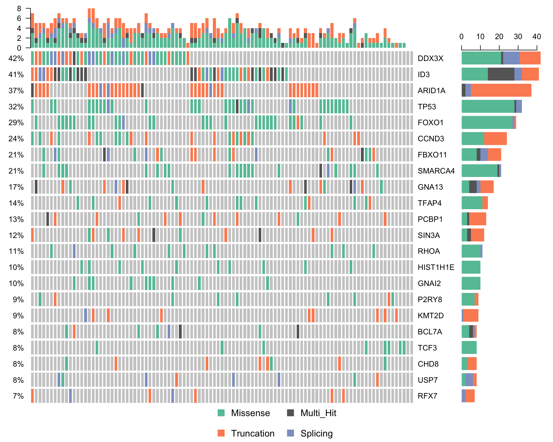
waterfallplot_maf <-
  subsetMaf(maf, query = "Variant_Classification %in% c('Truncation', 'Missense', 'Splicing')",
          mafObj = TRUE) %>%
  oncoplot(genes = smgs, colors = colours$categs, removeNonMutated = FALSE)
# print(waterfallplot_maf)
gprotein_genes <- c("GNA13", "P2RY8", "RHOA", "GNAI2", "ARHGEF40")

# maf@data %>%
#   filter(Hugo_Symbol %in% gprotein_genes) %>%
#   select(Hugo_Symbol, Tumor_Sample_Barcode) %>%
#   bind_rows(tibble(Hugo_Symbol = "DROP", Tumor_Sample_Barcode = unique(maf@data$Tumor_Sample_Barcode))) %>%
#   mutate(status = 0) %>%
#   distinct() %>%
#   spread(Hugo_Symbol, status, fill = 1, drop = FALSE) %>%
#   select(-Tumor_Sample_Barcode, -DROP) %>%
#   map(as.factor) %>%
#   table() %>%
#   c() %>%
#   cometExactTest::comet_exact_test()

oncostrip_maf_gproteins <- oncostrip(maf, genes = gprotein_genes,
                                     colors = colours$categs, removeNonMutated = FALSE)
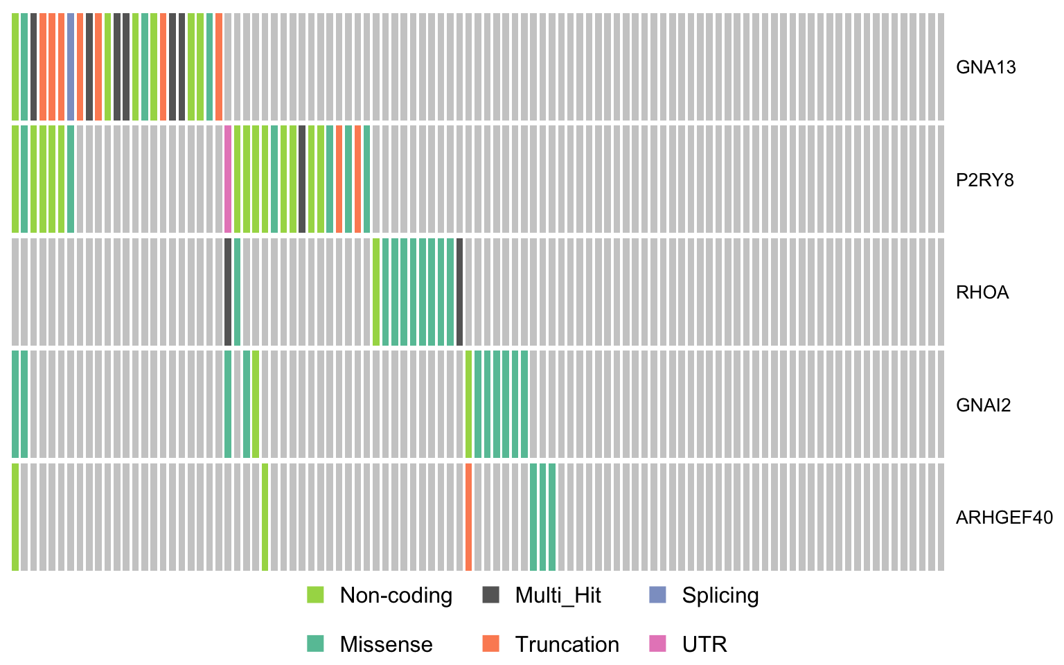
print(oncostrip_maf_gproteins)

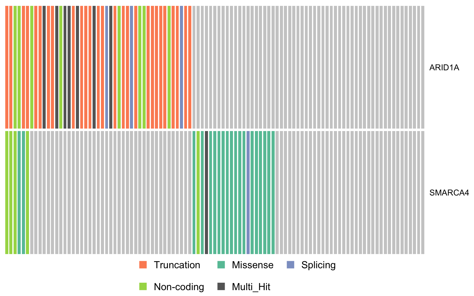
swisnf_genes <- c("ARID1A", "SMARCA4")

oncostrip_maf_swisnf <- oncostrip(
  maf, genes = swisnf_genes, colors = colours$categs, removeNonMutated = FALSE)

print(oncostrip_maf_swisnf)