Differential Gene Expression
Bruno Grande
2017-03-27
Differential Gene Expression
design(salmon$clean$dds) <- deseq_design
salmon$clean$dds         <- DESeq(salmon$clean$dds, minReplicatesForReplace = 5)
Tumour vs. Normal
Non-zero LFC
salmon$clean$de          <- list()
salmon$clean$de$ts       <- list()
salmon$clean$de$ts$lfc_0 <- results(
  salmon$clean$dds,
  contrast = list(c("clinical_variantSporadic", "clinical_variantEndemic"),
                  c("clinical_variantCentroblast")))

summary(salmon$clean$de$ts$lfc_0)
out of 36616 with nonzero total read count
adjusted p-value < 0.1
LFC > 0 (up)     : 10945, 30%
LFC < 0 (down)   : 9433, 26%
outliers [1]     : 0, 0%
low counts [2]   : 0, 0%
(mean count < 1)
[1] see 'cooksCutoff' argument of ?results
[2] see 'independentFiltering' argument of ?results plotMA(salmon$clean$de$ts$lfc_0, ylim = c(-5, 5))
Minimum 2 LFC
salmon$clean$de$ts$lfc_2 <- results(
  salmon$clean$dds,
  contrast = list(c("clinical_variantSporadic", "clinical_variantEndemic"),
                  c("clinical_variantCentroblast")),
  lfcThreshold = 2)

summary(salmon$clean$de$ts$lfc_2)
out of 36616 with nonzero total read count
adjusted p-value < 0.1
LFC > 0 (up)     : 782, 2.1%
LFC < 0 (down)   : 410, 1.1%
outliers [1]     : 0, 0%
low counts [2]   : 710, 1.9%
(mean count < 2)
[1] see 'cooksCutoff' argument of ?results
[2] see 'independentFiltering' argument of ?resultsplotMA(salmon$clean$de$ts$lfc_2, ylim = c(-5, 5))
plot_heatmap(salmon$clean$cvst[get_sig_genes(salmon$clean$de$ts$lfc_2),],
             colours, max_dim = 3000)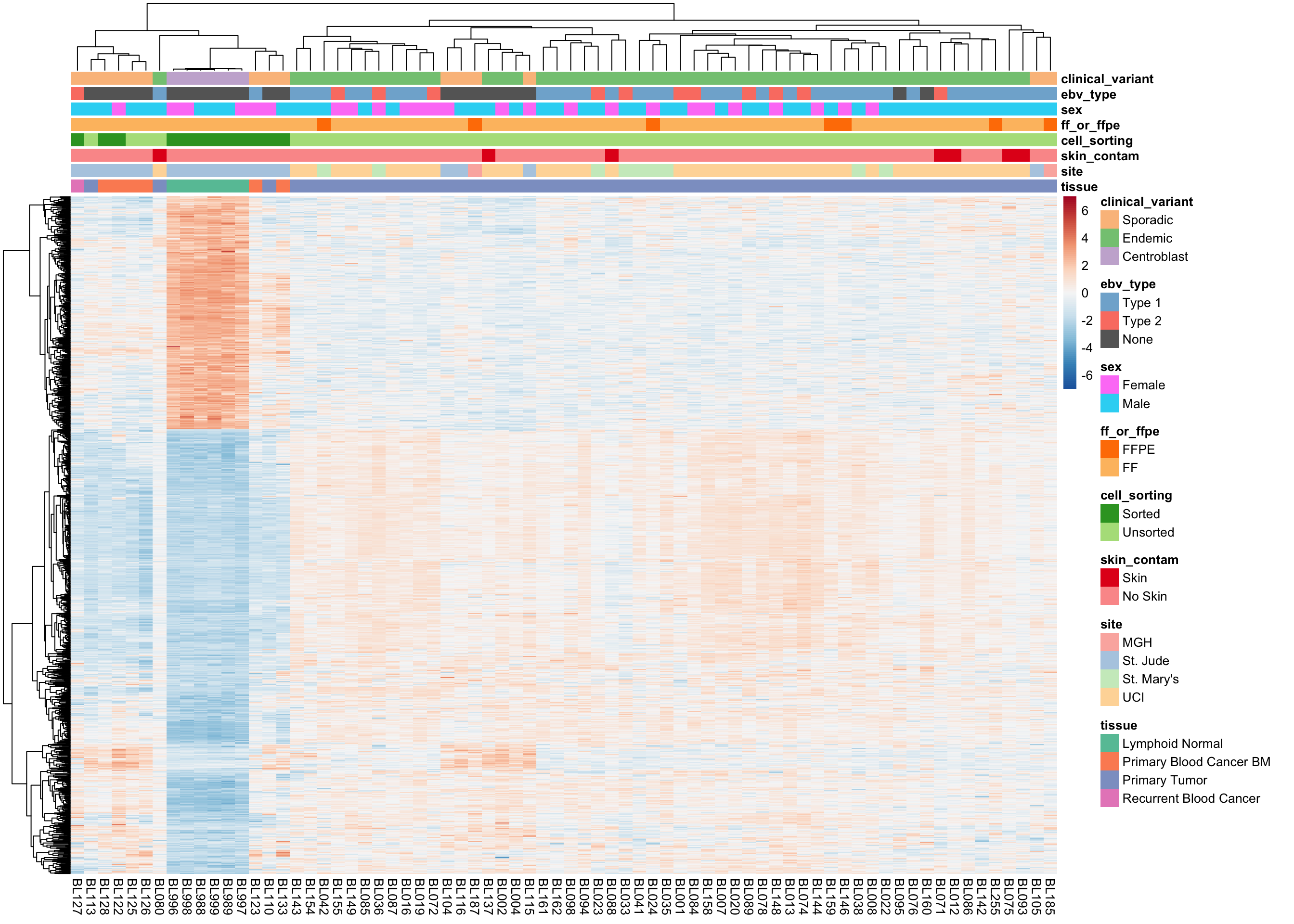
Endemic vs. Sporadic
Non-zero LFC
salmon$clean$de$cv$lfc_0 <- results(
  salmon$clean$dds,
  contrast = list(c("clinical_variantEndemic"),
                  c("clinical_variantSporadic")))

summary(salmon$clean$de$cv$lfc_0)
out of 36616 with nonzero total read count
adjusted p-value < 0.1
LFC > 0 (up)     : 3961, 11%
LFC < 0 (down)   : 4304, 12%
outliers [1]     : 0, 0%
low counts [2]   : 0, 0%
(mean count < 1)
[1] see 'cooksCutoff' argument of ?results
[2] see 'independentFiltering' argument of ?resultsplotMA(salmon$clean$de$cv$lfc_0, ylim = c(-5, 5))
Minimum 1.5 LFC
salmon$clean$de$cv$lfc_1.5 <- results(
  salmon$clean$dds,
  contrast = list(c("clinical_variantEndemic"),
                  c("clinical_variantSporadic")),
  lfcThreshold = 2)

summary(salmon$clean$de$cv$lfc_1.5)
out of 36616 with nonzero total read count
adjusted p-value < 0.1
LFC > 0 (up)     : 8, 0.022%
LFC < 0 (down)   : 12, 0.033%
outliers [1]     : 0, 0%
low counts [2]   : 1420, 3.9%
(mean count < 3)
[1] see 'cooksCutoff' argument of ?results
[2] see 'independentFiltering' argument of ?resultsplotMA(salmon$clean$de$cv$lfc_1.5, ylim = c(-5, 5))
plot_heatmap(salmon$clean$cvst[get_sig_genes(salmon$clean$de$cv$lfc_1.5),], colours)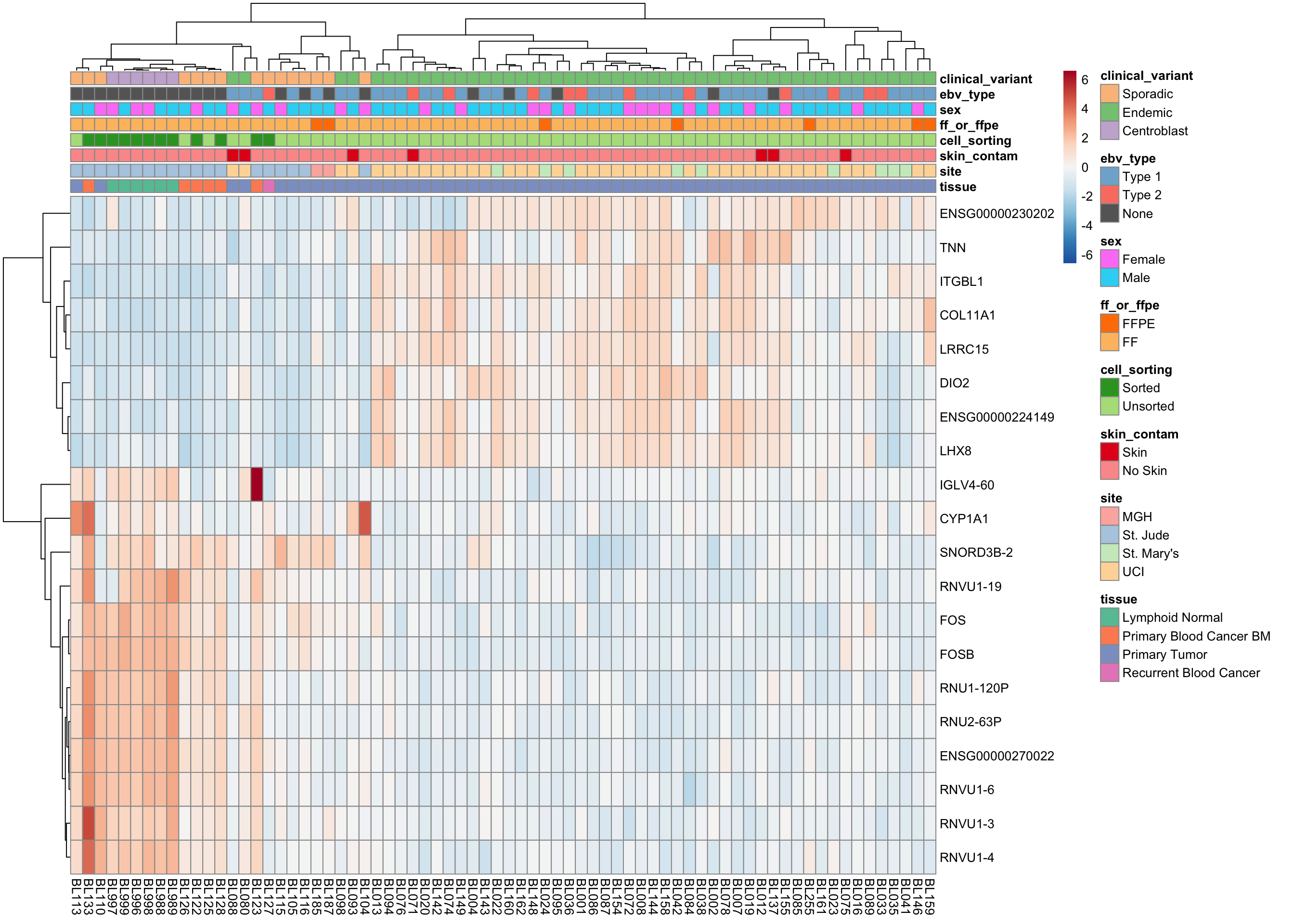
EBV-positive vs. EBV-negative
Non-zero LFC
salmon$clean$de$ebv$lfc_0 <- results(
  salmon$clean$dds,
  contrast = list(c("ebv_typeType.1", "ebv_typeType.2"),
                  c("ebv_typeNone")))

summary(salmon$clean$de$ebv$lfc_0)
out of 36616 with nonzero total read count
adjusted p-value < 0.1
LFC > 0 (up)     : 2264, 6.2%
LFC < 0 (down)   : 2194, 6%
outliers [1]     : 0, 0%
low counts [2]   : 1420, 3.9%
(mean count < 3)
[1] see 'cooksCutoff' argument of ?results
[2] see 'independentFiltering' argument of ?resultsplotMA(salmon$clean$de$ebv$lfc_0, ylim = c(-5, 5))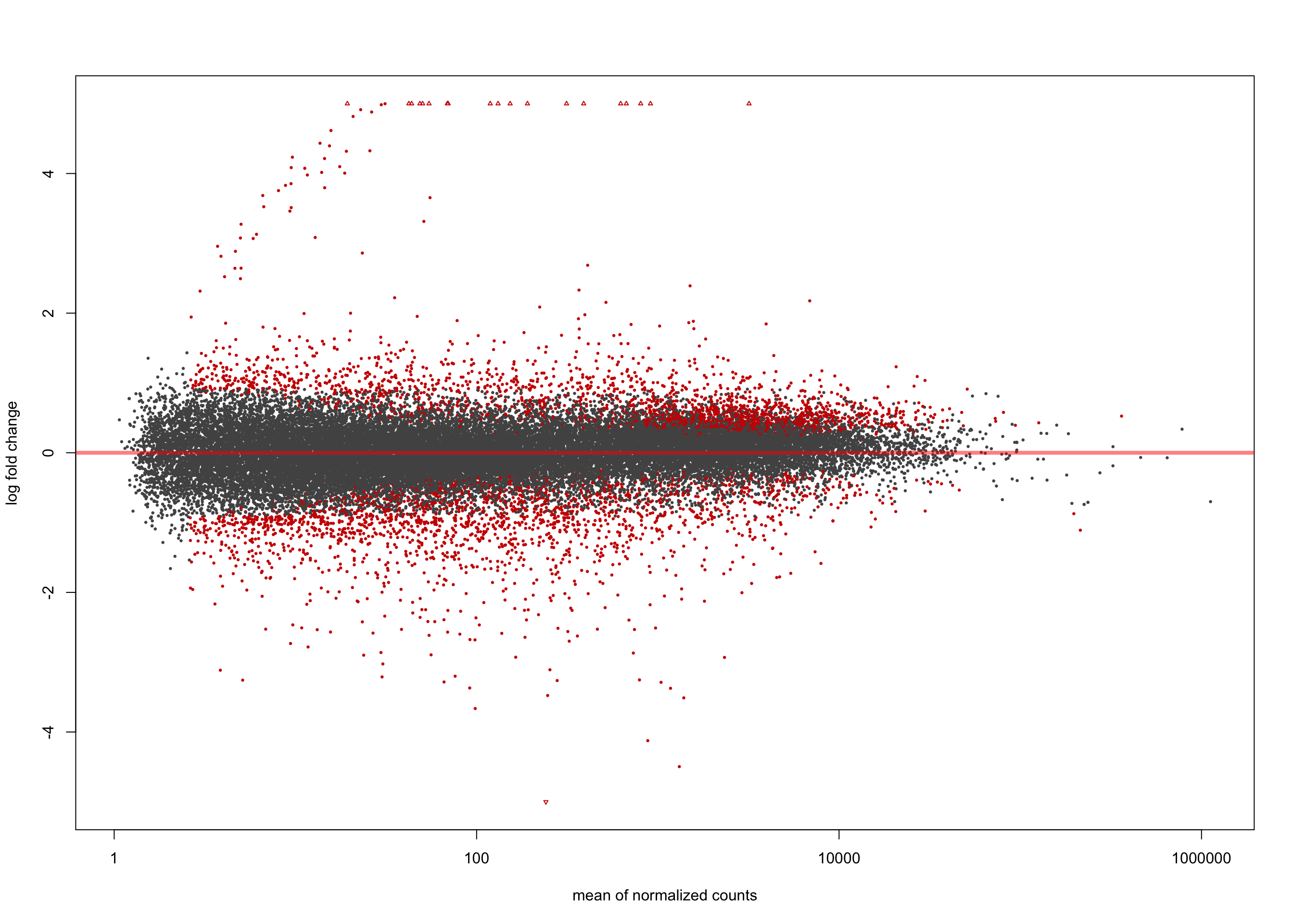
Minimum 1.5 LFC
salmon$clean$de$ebv$lfc_1.5 <- results(
  salmon$clean$dds,
  contrast = list(c("ebv_typeType.1", "ebv_typeType.2"),
                  c("ebv_typeNone")),
  lfcThreshold = 1.5)

summary(salmon$clean$de$ebv$lfc_1.5)
out of 36616 with nonzero total read count
adjusted p-value < 0.1
LFC > 0 (up)     : 56, 0.15%
LFC < 0 (down)   : 25, 0.068%
outliers [1]     : 0, 0%
low counts [2]   : 0, 0%
(mean count < 1)
[1] see 'cooksCutoff' argument of ?results
[2] see 'independentFiltering' argument of ?resultsplotMA(salmon$clean$de$ebv$lfc_1.5, ylim = c(-5, 5))
plot_heatmap(salmon$clean$cvst[get_sig_genes(salmon$clean$de$ebv$lfc_1.5),], colours)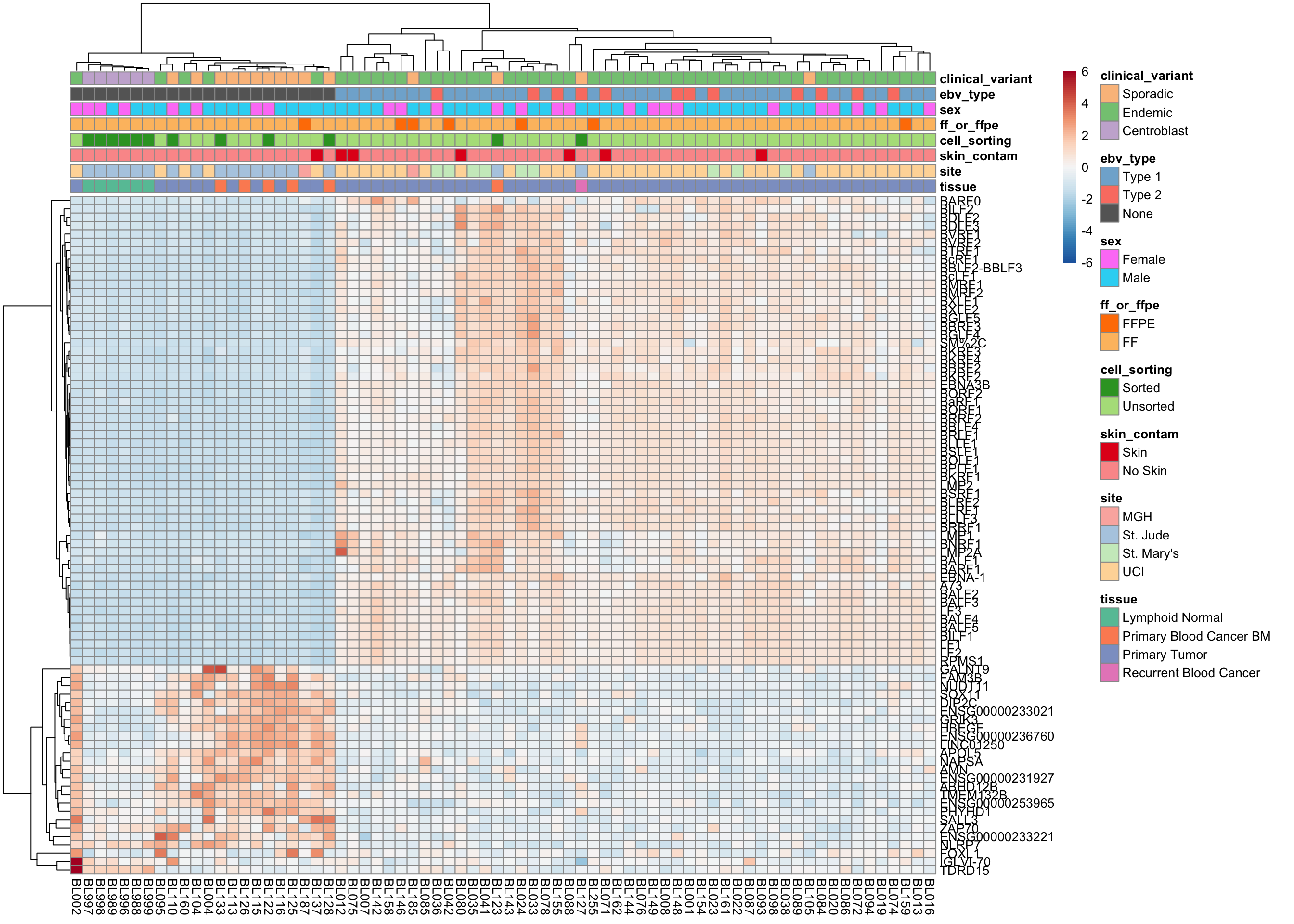
EBV Type 1 vs. EBV Type 2
Non-zero LFC
salmon$clean$de$ebvt$lfc_0 <- results(
  salmon$clean$dds,
  contrast = list(c("ebv_typeType.1"),
                  c("ebv_typeType.2")))

summary(salmon$clean$de$ebvt$lfc_0)
out of 36616 with nonzero total read count
adjusted p-value < 0.1
LFC > 0 (up)     : 13, 0.036%
LFC < 0 (down)   : 22, 0.06%
outliers [1]     : 0, 0%
low counts [2]   : 0, 0%
(mean count < 1)
[1] see 'cooksCutoff' argument of ?results
[2] see 'independentFiltering' argument of ?resultsplotMA(salmon$clean$de$ebvt$lfc_0, ylim = c(-5, 5))
plot_heatmap(salmon$clean$cvst[get_sig_genes(salmon$clean$de$ebvt$lfc_0),], colours)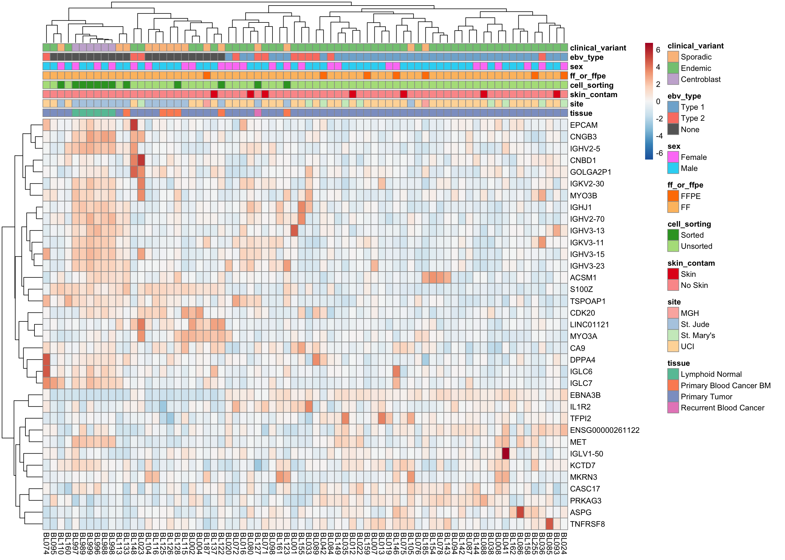
Gene-based Differential Gene Expression
tfs <- c("TFAP4", "SIN3A")
maf_patients <- unique(maf@data$patient)
salmon <- subset_salmon2(salmon, "muts", "clean", patients = maf_patients)

# Add mutation information to colData
colData(salmon$muts$dds) <-
  maf@data %>%
  filter(is_nonsynonymous(Consequence)) %>%
  select(patient, Hugo_Symbol) %>%
  distinct() %>%
  mutate(status = "mutated") %>%
  spread(Hugo_Symbol, status, fill = "unmutated") %>%
  arrange(match(patient, rownames(colData(salmon$muts$dds)))) %>%
  select(one_of(tfs)) %>%
  mutate_all(as.factor) %>%
  cbind(colData(salmon$muts$dds), .) %>%
  as.list() %>%
  map_if(is.factor, droplevels) %>%
  DataFrame()

muts_design <- paste0("~ sex + SV1 + SV2 + SV3 + ebv_type + clinical_variant + ",
                      paste(tfs, collapse = " + "))
design(salmon$muts$dds) <- as.formula(muts_design)
salmon$muts$dds <- DESeq(salmon$muts$dds, minReplicatesForReplace = 5)TFAP4
Non-zero LFC
salmon$muts$de$tfap4$lfc_0 <- results(
  salmon$muts$dds,
  contrast = list(c("TFAP4mutated"),
                  c("TFAP4unmutated")))

summary(salmon$muts$de$tfap4$lfc_0)
out of 36616 with nonzero total read count
adjusted p-value < 0.1
LFC > 0 (up)     : 4, 0.011%
LFC < 0 (down)   : 0, 0%
outliers [1]     : 0, 0%
low counts [2]   : 0, 0%
(mean count < 1)
[1] see 'cooksCutoff' argument of ?results
[2] see 'independentFiltering' argument of ?resultsplotMA(salmon$muts$de$tfap4$lfc_0, ylim = c(-5, 5))
USP7
Non-zero LFC
salmon$muts$de$sin3a$lfc_0 <- results(
  salmon$muts$dds,
  contrast = list(c("SIN3Amutated"),
                  c("SIN3Aunmutated")))

summary(salmon$muts$de$sin3a$lfc_0)
out of 36616 with nonzero total read count
adjusted p-value < 0.1
LFC > 0 (up)     : 43, 0.12%
LFC < 0 (down)   : 7, 0.019%
outliers [1]     : 0, 0%
low counts [2]   : 0, 0%
(mean count < 1)
[1] see 'cooksCutoff' argument of ?results
[2] see 'independentFiltering' argument of ?resultsplotMA(salmon$muts$de$sin3a$lfc_0, ylim = c(-5, 5))