Comparing Salmon and HTSeq
Bruno Grande
2017-02-18 14:30:26
Data Loading and Tidying
First, I load the Salmon quantification results. I use a transcript-to-gene map file to summarise the transcript counts at the gene level. Subsequently, I subset all expression matrices to the gene set common between the Salmon results and the htseq-count results.
# CDS only counts
salmon_cds_dir <- file.path(PROJHOME, "data", "salmon", "cds_only")
tx2gene_cds <- file.path(PROJHOME, "reference", "cds_transcript_gene.map")
salmon_cds <- load_salmon(salmon_cds_dir, tx2gene_cds)
counts_cds <- round(salmon_cds$counts)

# Full gene counts
salmon_full_dir <- file.path(PROJHOME, "data", "salmon", "full_gene")
tx2gene_full <- file.path(PROJHOME, "reference", "all_transcript_gene.map")
salmon_full <- load_salmon(salmon_full_dir, tx2gene_full)
counts_full <- round(salmon_full$counts)
counts_htseq_all <- set_rownames(expr, genes)
common_genes <- intersect(rownames(counts_cds), rownames(counts_htseq_all))
counts_cds <- counts_cds[common_genes, ]
counts_full <- counts_full[common_genes, ]
counts_htseq <- counts_htseq_all[common_genes, ]counts_df <-
dplyr::bind_rows(
expr_matrix_to_df(counts_cds, "salmon_cds"),
expr_matrix_to_df(counts_full, "salmon_full"),
expr_matrix_to_df(counts_htseq, "htseq_cds")) %>%
tidyr::spread(method, expr)NFKBIZ Expression
Read coverage in NFKBIZ was heavily skewed towards the 3’ end. This skewness was expected to affect the expression estimates. For this reason, we opted for CDS-only gene models for estimating expression using htseq-count.
I was interested in employing Salmon for estimating expression in order to include non-coding genes while using the latest genome build (GRCh38). However, the same concern persisted: will including untranslated regions (esp. UTRs) affect expression estimates?
Comparing gene models
In this analysis, I’m simply comparing NFKBIZ expression across all samples depending on whether which gene model was used for the Salmon quantification (CDS only or full gene).
nfkbiz_counts_df <-
  counts_df %>%
  dplyr::filter(gene == "NFKBIZ")

nfkbiz_cds_vs_full <-
  nfkbiz_counts_df %>%
  ggplot(aes(x = salmon_cds, y = salmon_full)) +
  geom_abline(slope = 1, colour = "dodgerblue", size = 1) +
  geom_point() +
  scale_x_log10() +
  scale_y_log10() +
  coord_fixed() +
  labs(
    title = "NFKBIZ Expression",
    x = "Salmon (CDS only; log scale)",
    y = "Salmon (full gene; log scale)")

nfkbiz_cds_vs_full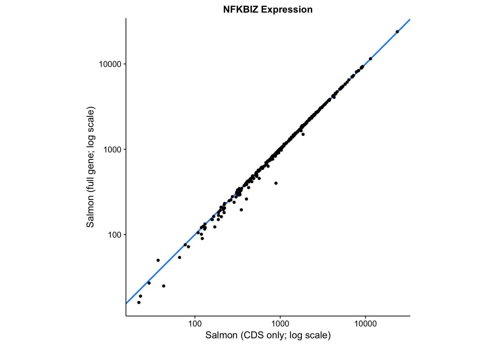
Visually, the correlation between the two gene models looks very good. Quantitatively, the Pearson correlation coefficient is 0.9997833, which is extremely high. In essence, Salmon seems to be robust to skewness in the read coverage across the gene. It properly handles the large number of reads aligned to the 3’UTR in the case of NFKBIZ.
Comparing quantification methods
After confirming that the gene model has little effect on the expression estimates produced by Salmon, I next wanted to see how well Salmon’s estimates agree with HTSeq’s for NFKBIZ.
nfkbiz_salmon_vs_htseq <-
  nfkbiz_counts_df %>%
  ggplot(aes(x = salmon_cds, y = htseq_cds)) +
  geom_abline(slope = 1, colour = "dodgerblue", size = 1) +
  geom_point() +
  scale_x_log10() +
  scale_y_log10() +
  coord_fixed() +
  labs(
    title = "NFKBIZ Expression",
    x = "Salmon (CDS only; log scale)",
    y = "HTSeq (CDS only; log scale)")

nfkbiz_salmon_vs_htseq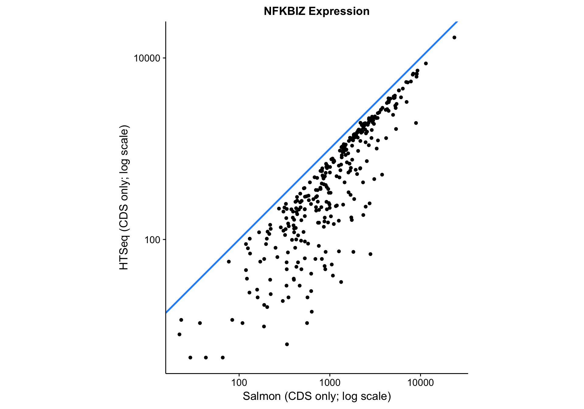
As you can see above, the correlation between methods is worse than between gene models. The Pearson correlation coefficient is not as bad as it seems due to the log scale: 0.9571582. Given that all data points lie below the identity line (y = x), HTSeq seems to be consistently underestimating expression compared to Salmon. It is unclear whether this is due to an increase in sensitivity or a decrease in specificity associated with Salmon.
One hint that the Salmon is more accurate than HTSeq is a blog post comparing the two methods using simulated data.
HTSeq versus ground truth
Compared to ground truth, HTSeq seems to underestimate the expression for several genes. You can also notice that there is an association between underestimating expression and low fraction of unique sequence in the gene. This is consistent with the fact that HTSeq ignores multi-mapped reads.

HTSeq versus ground truth
Salmon versus ground truth
On the other hand, Salmon handles the low fraction of unique sequence much better than HTSeq.

Salmon versus ground truth
A peer-reviewed paper showed that aggregating transcript-level counts (e.g. with Salmon) outperforms gene-level counting methods (e.g. HTSeq) for differential gene expression analysis.
Genome-wide Expression
After inspecting how different gene models and methods affect NFKBIZ expression, I am curious about their effects genome-wide. Because of the higher dimensionality, I am
Comparing gene models
Patient level
cds_vs_full_patient_cor_df <-
  counts_df %>%
  dplyr::group_by(patient) %>%
  dplyr::summarise(pearson = cor(salmon_cds, salmon_full, method = "pearson"),
                   spearman = cor(salmon_cds, salmon_full, method = "spearman"))

cds_vs_full_patient_cor_plot <-
  cds_vs_full_patient_cor_df %>%
  ggplot(aes(x = pearson, y = spearman, label = patient)) +
  geom_point() +
  labs(title = "Correlation coefficients between patients\nComparing gene models using Salmon")

cds_vs_full_patient_cor_plot
Gene level
cds_vs_full_gene_cor_df <-
  counts_df %>%
  dplyr::group_by(gene) %>%
  dplyr::mutate(min_median = min(median(salmon_cds), median(salmon_full))) %>%
  dplyr::filter(min_median > 1) %>%
  dplyr::summarise(pearson = cor(salmon_cds, salmon_full, method = "pearson"),
                   spearman = cor(salmon_cds, salmon_full, method = "spearman"))

cds_vs_full_gene_cor_plot <-
  cds_vs_full_gene_cor_df %>%
  ggplot(aes(x = pearson, y = spearman, label = gene)) +
  geom_point() +
  labs(title = "Correlation coefficients between genes\nComparing gene models using Salmon")

cds_vs_full_gene_cor_plot
Comparing quantification methods
Patient level
salmon_vs_htseq_patient_cor_df <-
  counts_df %>%
  dplyr::group_by(patient) %>%
  dplyr::summarise(pearson = cor(salmon_cds, htseq_cds, method = "pearson"),
                   spearman = cor(salmon_cds, htseq_cds, method = "spearman"))

salmon_vs_htseq_patient_cor_plot <-
  salmon_vs_htseq_patient_cor_df %>%
  ggplot(aes(x = pearson, y = spearman, label = patient)) +
  geom_point() +
  labs(title = "Correlation coefficients between patients\nComparing Salmon and HTSeq")

salmon_vs_htseq_patient_cor_plot
Gene level
salmon_vs_htseq_gene_cor_df <-
  counts_df %>%
  dplyr::group_by(gene) %>%
  dplyr::mutate(min_median = min(median(salmon_cds), median(htseq_cds))) %>%
  dplyr::filter(min_median > 1) %>%
  dplyr::summarise(pearson = cor(salmon_cds, htseq_cds, method = "pearson"),
                   spearman = cor(salmon_cds, htseq_cds, method = "spearman"))

salmon_vs_htseq_gene_cor_plot <-
  salmon_vs_htseq_gene_cor_df %>%
  ggplot(aes(x = pearson, y = spearman, label = gene)) +
  geom_point() +
  labs(title = "Correlation coefficients between genes\nComparing Salmon and HTSeq")

salmon_vs_htseq_gene_cor_plot