Predicting COO Using RNA-seq Data
Bruno Grande
2017-02-18 13:48:22
Most Variably Expressed Genes
For unsupervised clustering, typically only the most variably expressed genes are considered. There are multiple approaches to determining variability. The most common is to simply use variance. I was initially concerned that using raw variance would bias the selection towards more highly expressed genes, because higher expression values generally results in higher absolute variance values. Therefore, I was thinking of using the coefficient of variation instead.
However, if you compare gene expression before and after DESeq2 variance-stabilizing transformation, as expected, the relationship between the mean and variance is greatly reduced. Therefore, the need to normalize for mean expression is also greatly reduced.
scatterplot_expr_gene_mean_sd$labels$title <- "Raw expression counts per gene"

scatterplot_expr_gene_mean_sd$layers[3] <- NULL

scatterplot_texpr_gene_mean_sd <-
  scatterplot_expr_gene_mean_sd %+% texpr_gene_stats +
  labs(title = "Transformed expression counts per gene")

scatterplot_compare_expr_texpr <-
  cowplot::plot_grid(scatterplot_expr_gene_mean_sd, scatterplot_texpr_gene_mean_sd)

scatterplot_compare_expr_texpr
That being said, variance is susceptible to outliers. A more robust measure of variability is the median absolute deviation about the median, or MAD. The formula for MAD is:
\[MAD = median( |X_i - median(X)| )\]
Because we are interested in exploring existing subtypes that should affect most samples, we aren’t as interested in variation that only arises in few samples (i.e. outliers). Hence, I will be using MAD as the metric for variability.
First, we will select the most variably expressed genes based on this metric.
top_mad <- most_mad(texpr, 0.25)
texpr_top_mad <- texpr[top_mad, ]
Let’s quickly explore the properties of the selected genes relative to other genes. As we would expect, the selected genes are among those with the highest standard deviation (SD). However, there are a number of genes with high SD but have not been selected. This is most likely due to the robustness of MAD to outliers. Presumably, the high-SD genes that were not selected have high SD because of a few outlier samples.
texpr_gene_stats$selected <- "No"
texpr_gene_stats[top_mad, "selected"] <- "Yes"

scatterplot_texpr_gene_mean_sd_highlight_top_mad <-
  dplyr::filter(texpr_gene_stats, selected == "No") %>%
  ggplot(aes(x = mean, y = sd, colour = selected, text = gene)) +
  geom_point(alpha = 0.5) +
  geom_point(data = dplyr::filter(texpr_gene_stats, selected == "Yes"),
             alpha = 0.5) +
  scale_color_manual(values = c(No = "grey", Yes = "red"), name = "Among selected?") +
  place_legend(c(1,1)) +
  labs(title = "Mean and SD of expression of selected versus other genes",
       x = "Mean", y = "SD")

scatterplot_texpr_gene_mean_sd_highlight_top_mad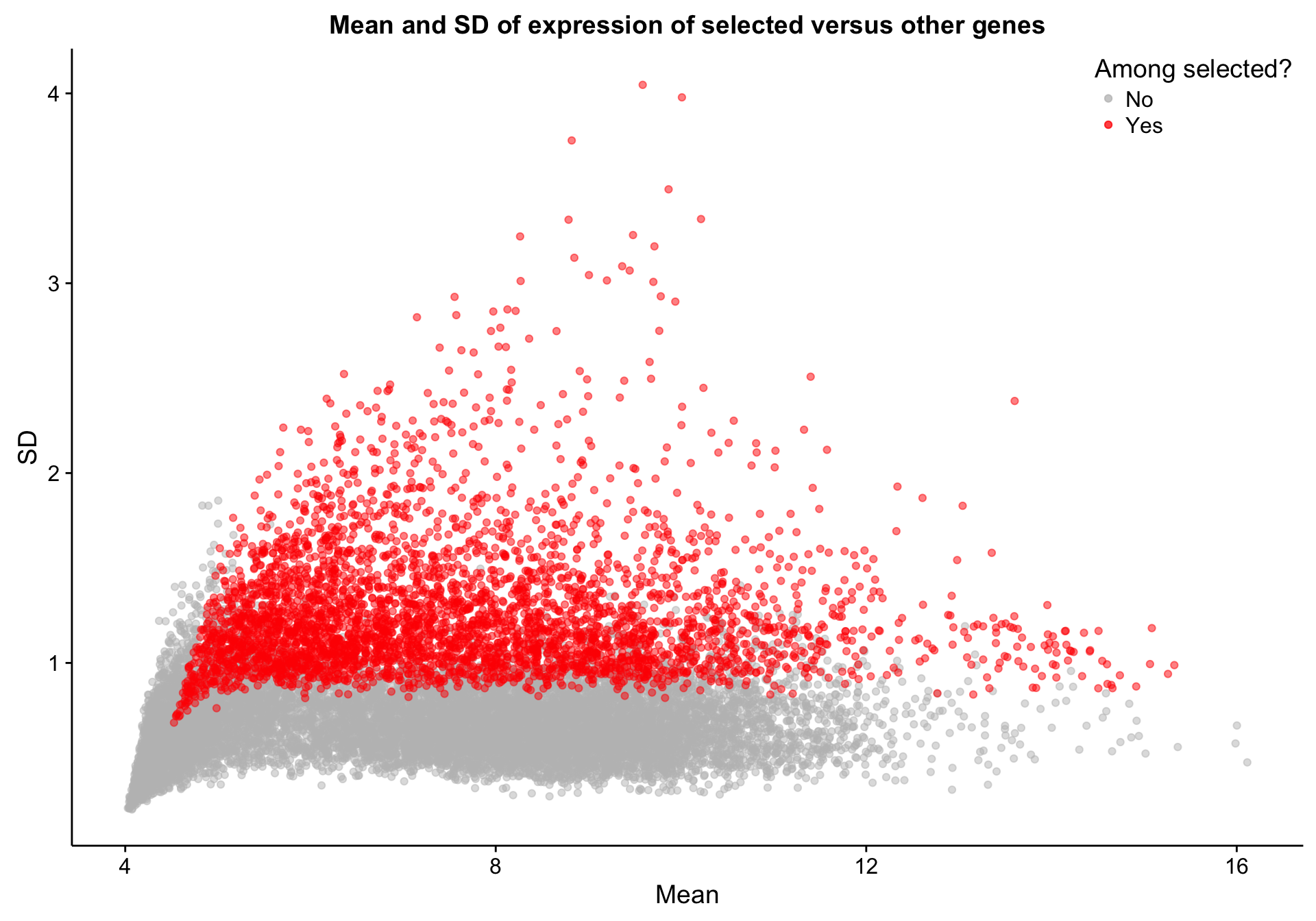
Unsupervised Clustering
Most Variably Expressed Genes
Now that we have selected the 500 most variably expressed genes, we can perform unsupervised clustering using different methods.
Principle component analysis
Principle component analysis on the 500 most variably expressed genes (defined by MAD) shows mild clustering on the NanoString COO status (coo_ns), explained by PC2.
pca_data <- calc_pca(tdds, intgroup = "coo_ns", ntop = ntop)

pca_percentVar <- attr(pca_data, "percentVar")

cat(paste0("Variance explained by PC1: ", round(pca_percentVar[1]*100, 1), "%"),
    paste0("Variance explained by PC2: ", round(pca_percentVar[2]*100, 1), "%"),
    sep = "\n")
Variance explained by PC1: 42.6%
Variance explained by PC2: 6.1%pca_texpr <-
ggplot2::ggplot(pca_data, aes(x = PC1, y = PC2, colour = coo_ns)) +
geom_point(data = dplyr::select(pca_data, -coo_ns),
size = 2, colour = "grey", alpha = 0.5) +
geom_point(size = 2) +
scale_colour_manual(values = colours$coo) +
labs(title = paste0("Principle component analysis (PCA)\n",
"According to the ", ntop, " most variable genes\n",
"Split by Lymph2Cx COO status"),
colour = "Cell-of-origin")
pca_texpr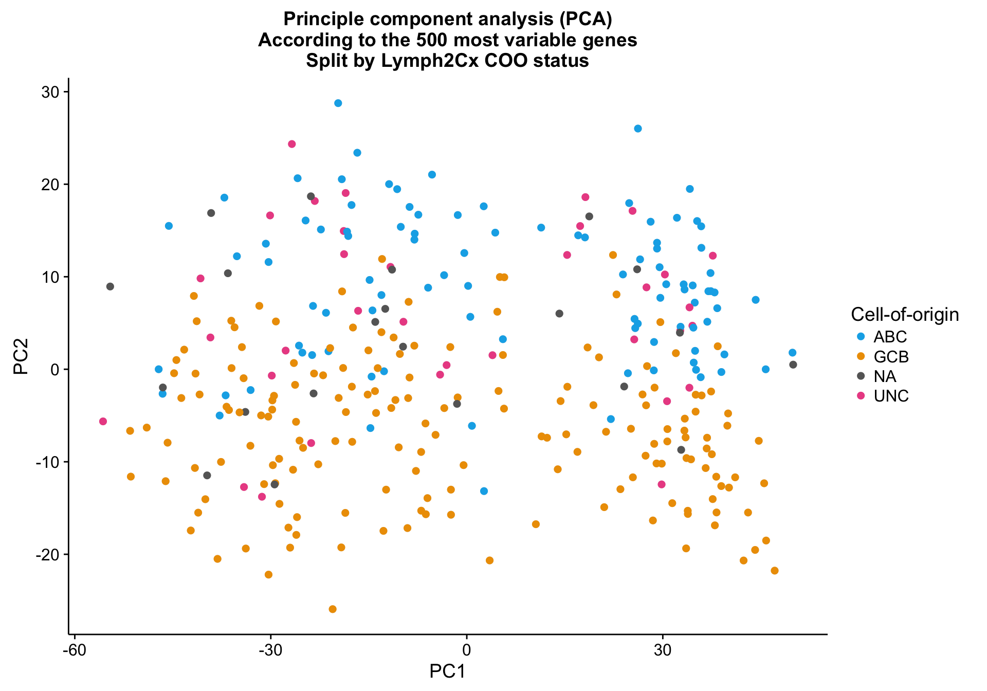
pca_texpr_split <-
  pca_texpr +
  facet_wrap(~coo_ns) +
  scale_colour_manual(values = colours$coo, breaks = NULL)
pca_texpr_split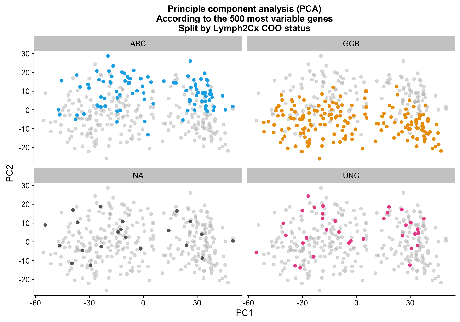
Hierarchical clustering
While samples with the same Lymph2Cx COO status tend to cluster together, there are larger sources of variation that prevent COO clustering cohort-wide.
hm_annot <- coo[,-1, drop = FALSE]

plot_heatmap(texpr_top_mad, hm_annot, annotation_colors = colours)
Non-negative matrix factorization
Selecting the best rank
nmf_top_mad_rank_survey <- NMF::nmf(texpr_top_mad, 2:5, nrun = 30, seed = global_seed)
plot(nmf_top_mad_rank_survey)![]()
coo_annot_mut <-
  coo %>%
  extract(colnames(texpr_top_mad), ) %>%
  dplyr::left_join(tibble::rownames_to_column(heatmap_mut_rf_prob_annot, "patient")) %>%
  tidyr::replace_na(list(gcb_num_feats = "NA", abc_num_feats = "NA", abc_gcb_diff = "NA")) %>%
  tibble::column_to_rownames("patient")

anno.simple = coo_annot_mut[,"coo_ns", drop = FALSE]
anno.simple$coo_ns[anno.simple$coo_ns == "NA"] = "UNC"
NMF::consensusmap(nmf_top_mad_rank_survey, annCol = anno.simple,
labCol = NA, labRow = NA, annColors = colours)![]()
Wright et al. genes
A good sanity check of the NanoS tring COO assignments is to cluster while only using genes whose expression define COO. For this, we are using genes reported by Wright et al.. There are several unsupervised clustering methods available to us.
Hierarchical clustering
Hierarchical clustering of the Wright genes is much better at separating ABC and GCB DLBCL cases (assuming the NanoString COO status is correct).
texpr_wright <- texpr[gene_ids_filt %in% gene_ids$wright, ]
genes_wright <- genes[match(gene_ids$wright, gene_ids$rnaseq)]

pheatmap_wright_hclust <- plot_heatmap(texpr_wright, hm_annot, colours)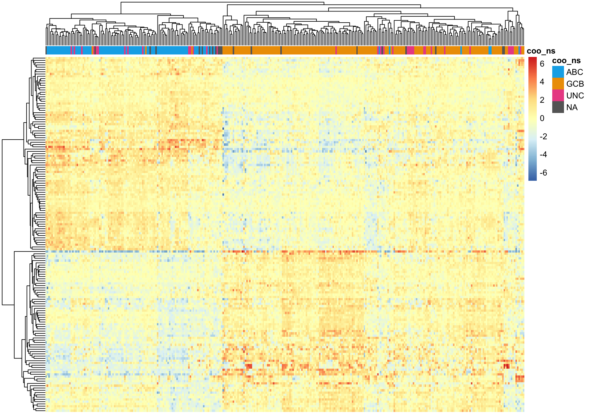
K-means clustering
On the other hand, k-means clustering performs very poorly.
wright_kmeans <- kmeans(t(texpr_wright), 2)

pheatmap_wright_kmeans <- plot_heatmap(texpr_wright[, order(wright_kmeans$cluster)],
                                       hm_annot, colours, cluster_cols = FALSE)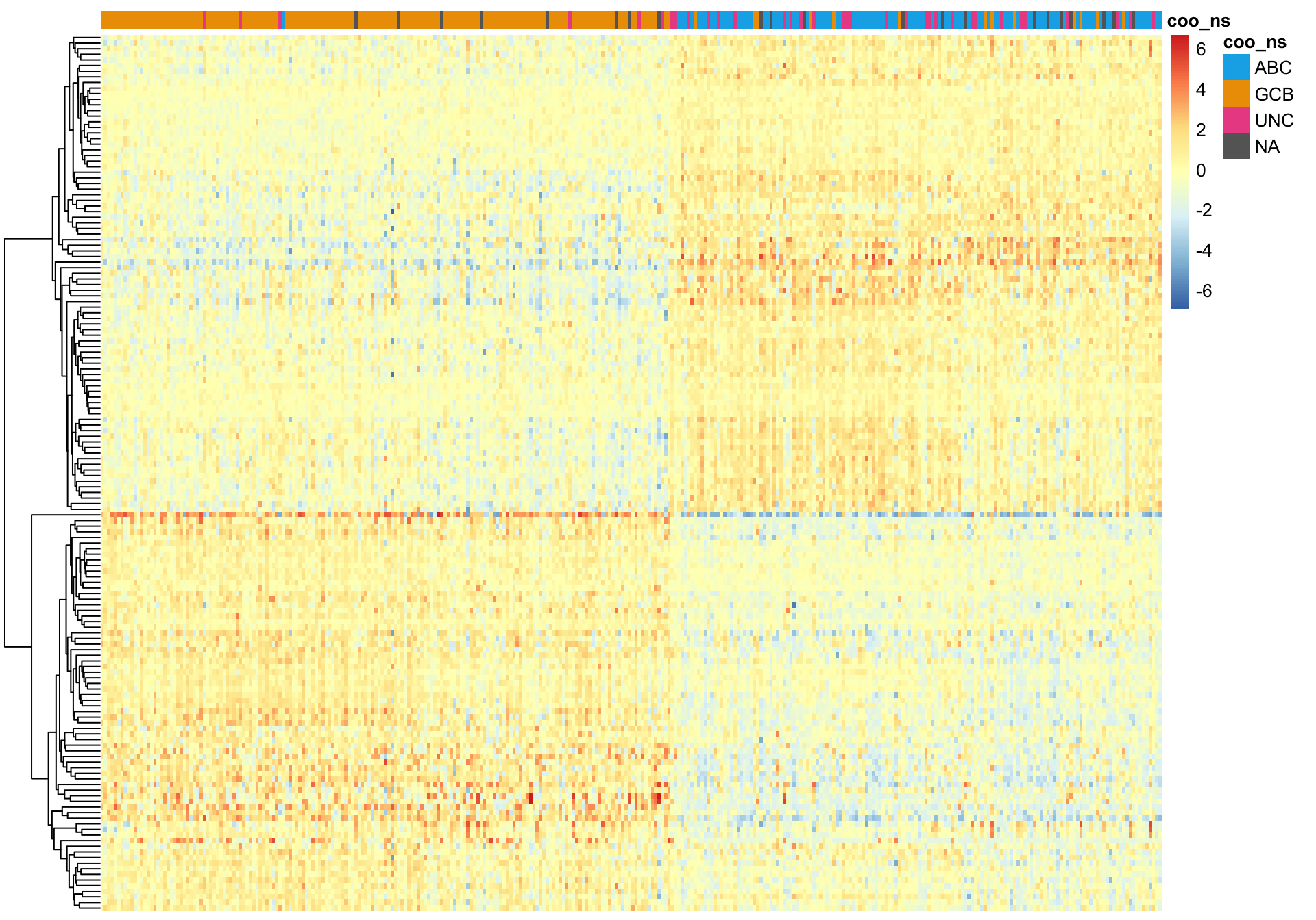
Principle component analysis
PCA on the Wright genes definitely separates the ABC and GCB cases with some overlap remaining. Furthermore, the NA cases are spread out across the PCA plot, while the UNC cases are clearly located at the interface between ABC and GCB, which is expected.
pca_wright_data <- DESeq2::plotPCA(tdds[gene_ids_filt %in% gene_ids$wright, ],
                                   intgroup = "coo_ns", returnData = TRUE)

pca_wright <-
  ggplot2::ggplot(pca_wright_data, aes(x = PC1, y = PC2, colour = coo_ns)) +
  geom_point(data = dplyr::select(pca_wright_data, -coo_ns),
             size = 2, colour = "grey", alpha = 0.5) +
  geom_point(size = 2) +
  scale_colour_manual(values = colours$coo) +
  labs(title = paste0("Principle component analysis (PCA)\n",
                      "Restricted to Wright et al. genes\n",
                      "Split by Lymph2Cx COO status"))
pca_wright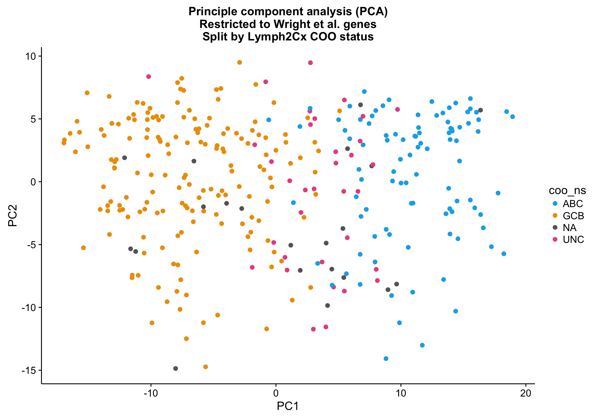
pca_wright_split <-
  pca_wright +
  facet_wrap(~coo_ns) +
  scale_colour_manual(values = colours$coo, breaks = NULL)
pca_wright_split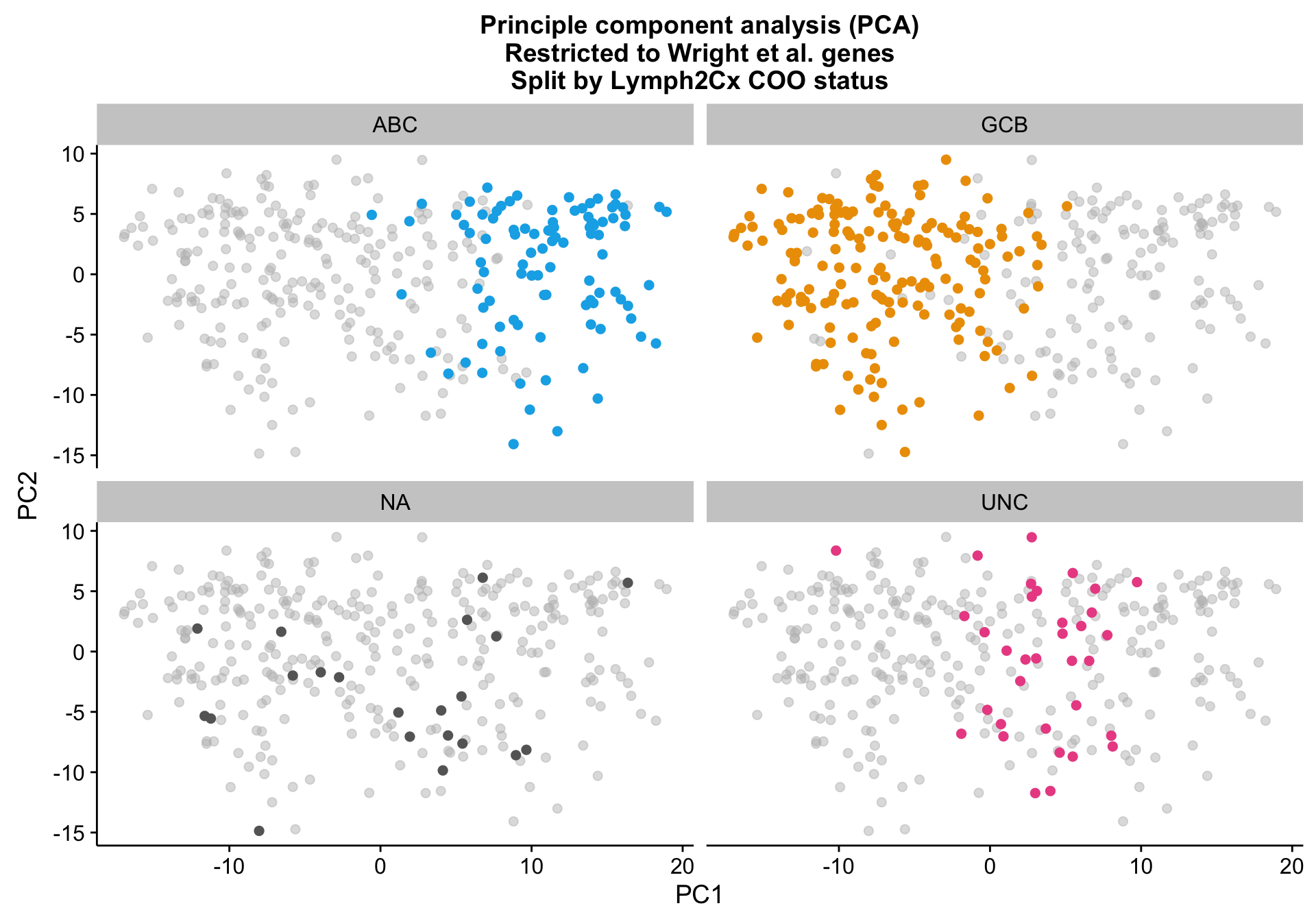
Non-negative matrix factorization
Selecting the best rank
nmf_wright_rank_survey <- NMF::nmf(texpr_wright, 2:5, nrun = 50, seed = global_seed)
plot(nmf_wright_rank_survey)![]()
NMF::consensusmap(nmf_wright_rank_survey, annCol = coo_annot_mut,
labCol = NA, labRow = NA, annColors = colours)![]()
nmf_wright_method_survey <- NMF::nmf(texpr_wright, 2, list("brunet", "lee", "ns"),
                                     nrun = 50, seed = global_seed, .options = "t")
Compute NMF method 'brunet' [1/3] ... OK
Compute NMF method 'lee' [2/3] ... OK
Compute NMF method 'ns' [3/3] ... OKplot(nmf_wright_method_survey)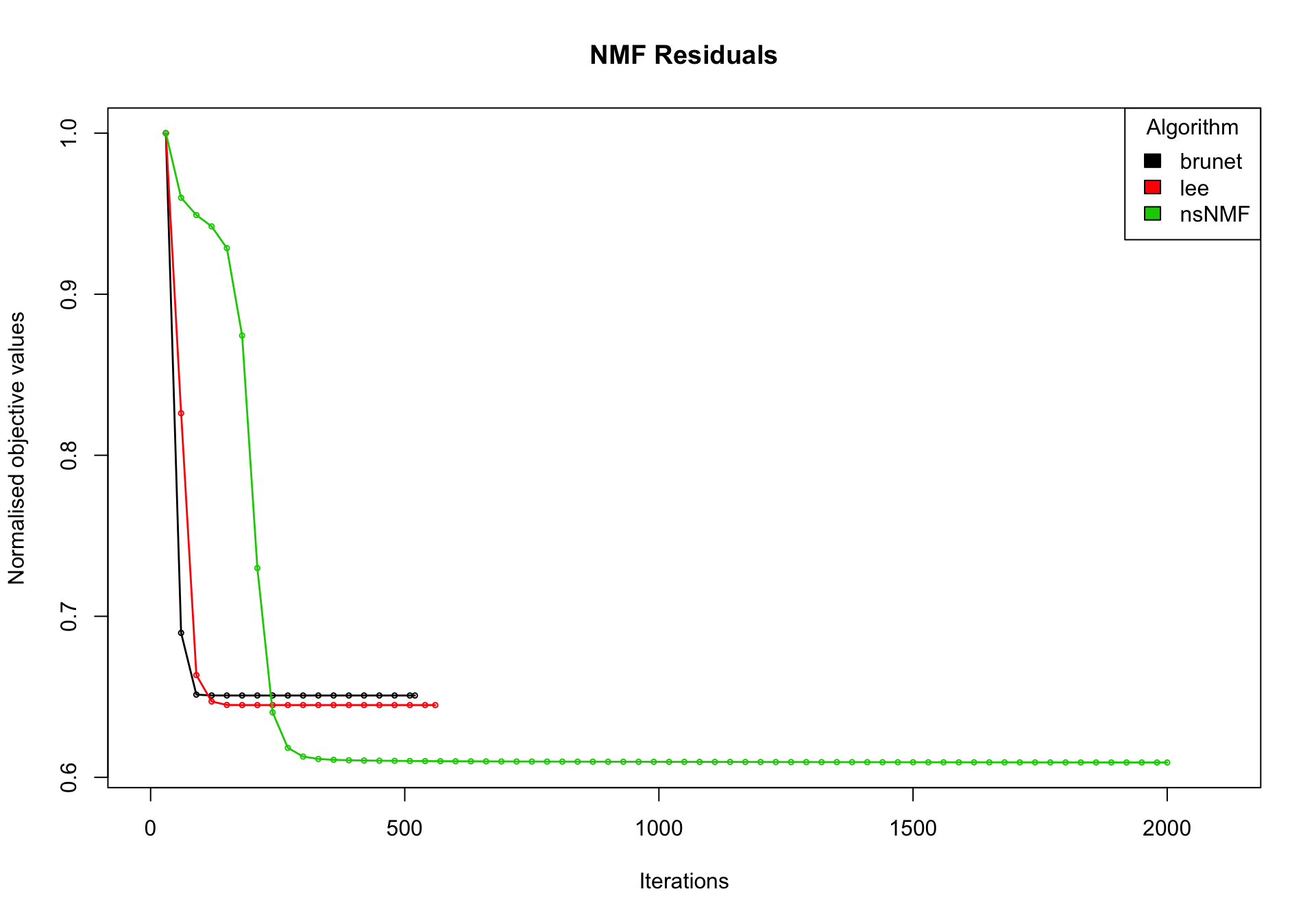
NMF::consensusmap(nmf_wright_method_survey, annCol = coo_annot_mut,
                  labCol = NA, labRow = NA, annColors = colours)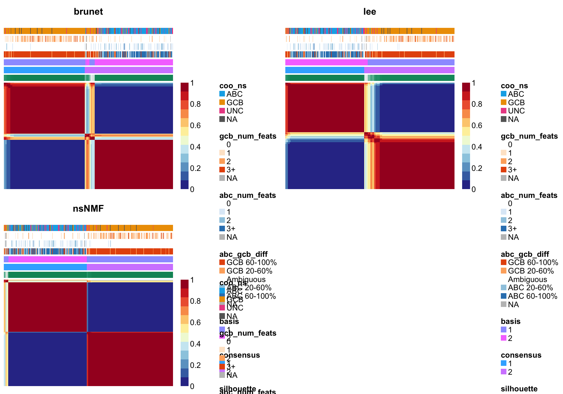
nmf_wright <- NMF::nmf(texpr_wright, 2, "brunet", nrun = 250, seed = global_seed)
NMF::consensusmap(nmf_wright, labCol = NA, labRow = NA,
                  annCol = coo_annot_mut, annColors = colours)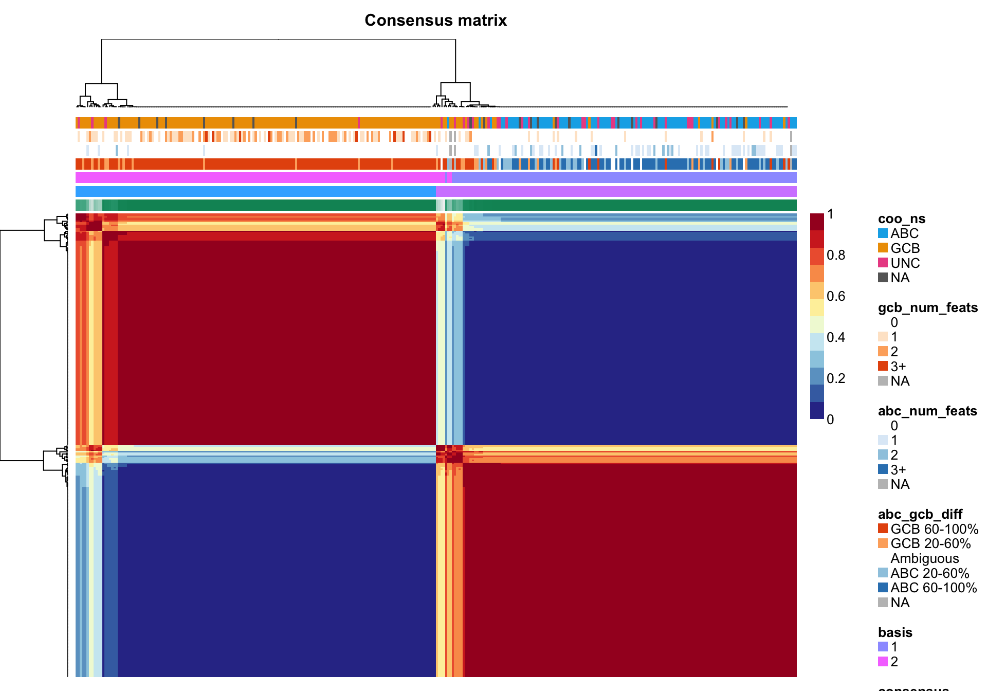
NMF::basismap(nmf_wright, subsetRow = TRUE)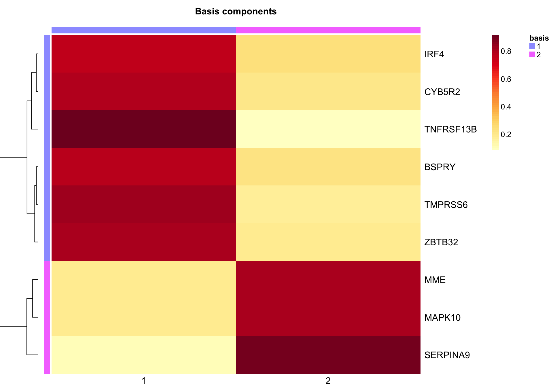
NMF::coefmap(nmf_wright, distfun = "correlation",
             annCol = coo_annot_mut, annColors = colours)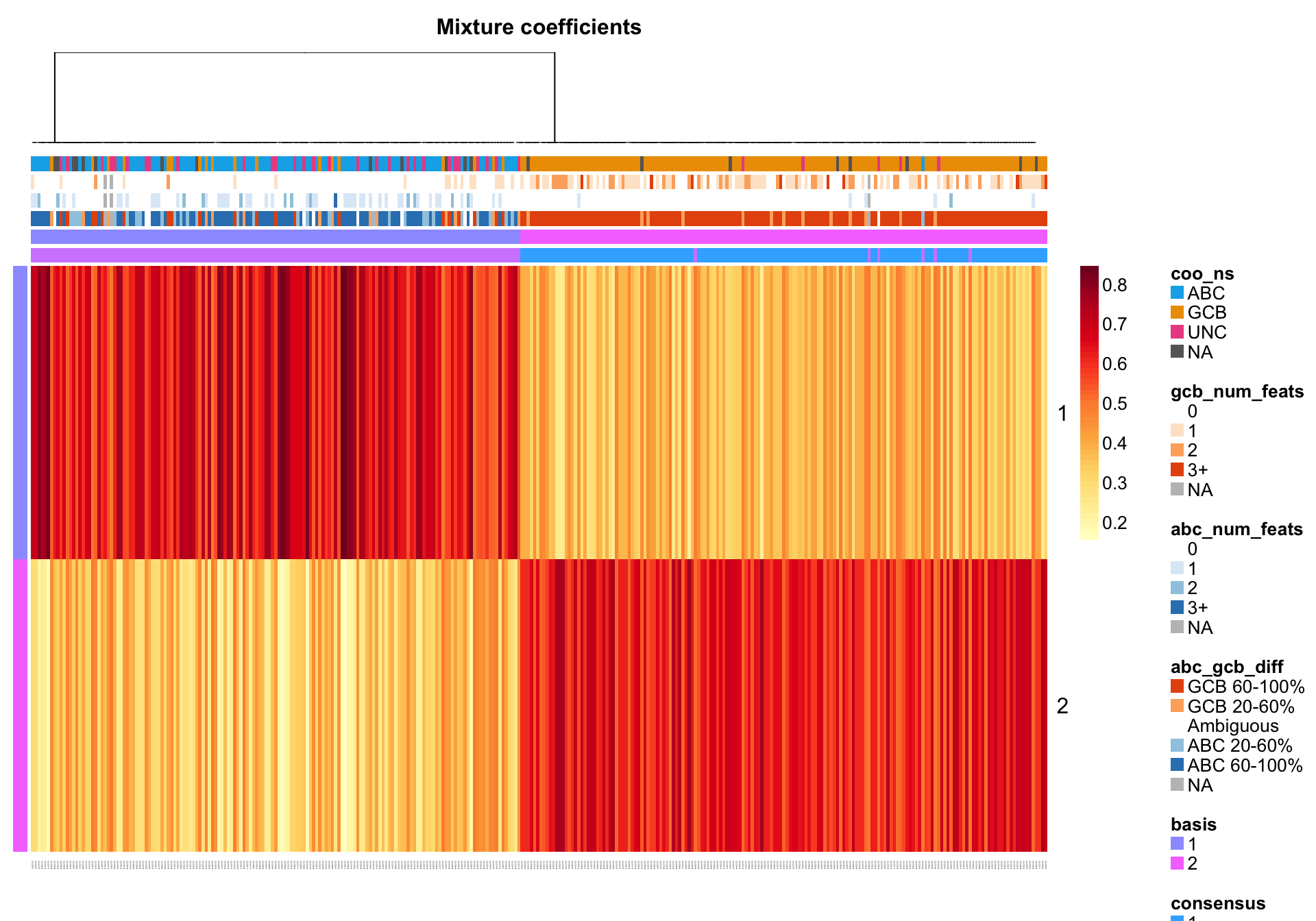
nmf_wright_features_kim <- NMF::extractFeatures(nmf_wright, "kim")
nmf_wright_fscores_kim <- NMF::featureScore(nmf_wright, "kim")

metagene1_kim <- genes_wright[nmf_wright_features_kim[[1]]]
metagene2_kim <- genes_wright[nmf_wright_features_kim[[2]]]
Using the “kim” method, the basis 1 metagene consists of the following genes: TNFRSF13B, TMPRSS6, ZBTB32, CYB5R2, BSPRY, IRF4.
The basis 2 metagene consists of the following genes: SERPINA9, MME, MAPK10
nmf_wright_features_max <- NMF::extractFeatures(nmf_wright, "max")
nmf_wright_fscores_max <- NMF::featureScore(nmf_wright, "max")

metagene1_max <- genes_wright[nmf_wright_features_max[[1]]]
metagene2_max <- genes_wright[nmf_wright_features_max[[2]]]
Using the “max” method, the basis 1 metagene consists of the following genes: HSP90B1, BATF, TNFRSF13B, KIAA0226L, IL16, PTPN1, FOXP1, HCK, SUB1, PIM2_ENSG00000102096, CFLAR, PDLIM1, MPEG1, ERP29, CARD11, CLECL1, CCDC50, ARHGAP17, TCF4, DOCK10, BLNK_ENSG00000095585, IRF4, SSR3, GNL3, COPB2, CYB5R2, TGIF1, MRPL3, ENTPD1, FUT8, SH3BP5, PIM1, TOX2, TBL1XR1, TARS, TNFAIP8, CLINT1, CCND2, NFKBIZ, CSNK1E, NIPA2, NRROS, STAMBPL1, RILPL2, SLA, ARID3A, ETV6, RAB7L1, ARHGAP24, RASGRF1, LMAN1, TCTN3.
The basis 2 metagene consists of the following genes: SERPINA9, SEL1L3, MME, LRMP, MARCKSL1, BCL6, STAG3, DNAJC10, MYBL1, HDAC1, ZNF318, STK17A, ANKRD13A, TMEM123, LMO2, PLEKHF2, SMARCA4, SSBP2, NEK6, PTK2, DENND3, CDK14, BAZ2B
nmf_prob <- predict(nmf_wright, prob = TRUE)

coo_annot_mut_nmf <-
  coo_annot_mut %>%
  tibble::rownames_to_column("patient") %>%
  dplyr::bind_cols(nmf_prob) %>%
  dplyr::rename(nmf_class = predict, nmf_prob = prob) %>%
  dplyr::mutate(nmf_threshold = ifelse(nmf_prob > 0.55, "Pass", "Fail")) %>%
  as.data.frame() %>%
  tibble::column_to_rownames("patient")
coo_annot_mut_nmf <- coo_annot_mut_nmf[
colnames(texpr_wright) , c("coo_ns", "abc_gcb_diff", "nmf_class", "nmf_threshold")]
pheatmap_nmf_metagenes_max <- plot_heatmap(texpr_wright[c(metagene1_max, metagene2_max), ],
coo_annot_mut_nmf, colours, cutree_cols = 3,
clustering_distance_cols = 'correlation')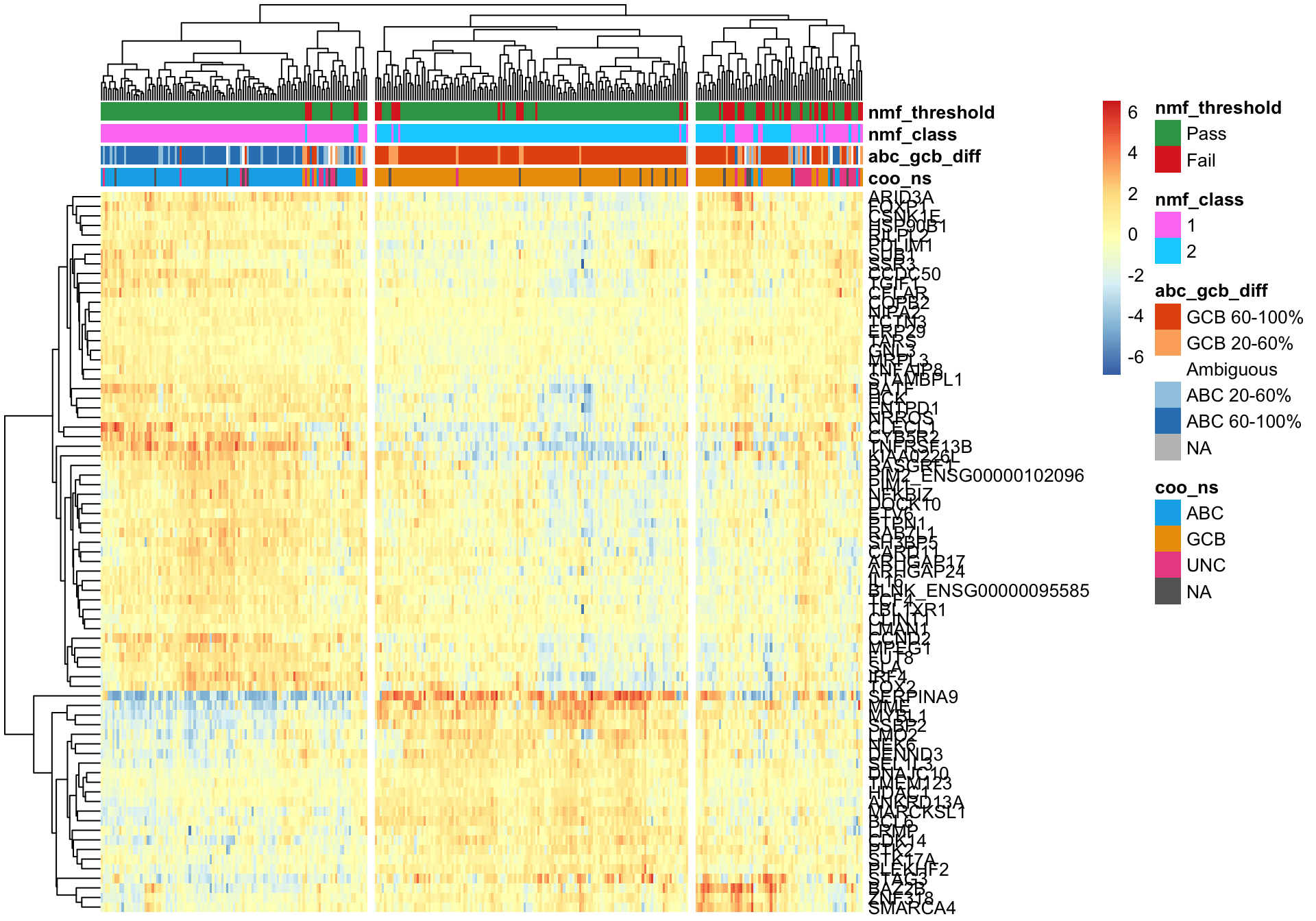
passed <- coo_annot_mut_nmf$nmf_threshold == "Pass"
pheatmap_nmf_metagenes_max <- plot_heatmap(texpr_wright[c(metagene1_max, metagene2_max), passed],
                                           coo_annot_mut_nmf[passed, ], colours, cutree_cols = 2,
                                           clustering_distance_cols = 'correlation')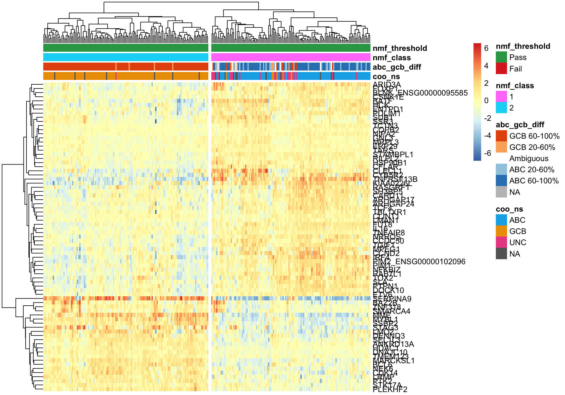
Lymph2Cx genes
Hierarchical clustering
And the same can be done using the genes on the Lymph2cx NanoString assay.
texpr_lymph2cx <- texpr[gene_ids_filt %in% gene_ids$lymph2cx, ]

plot_heatmap(texpr_lymph2cx, coo_annot_mut, annotation_colors = colours)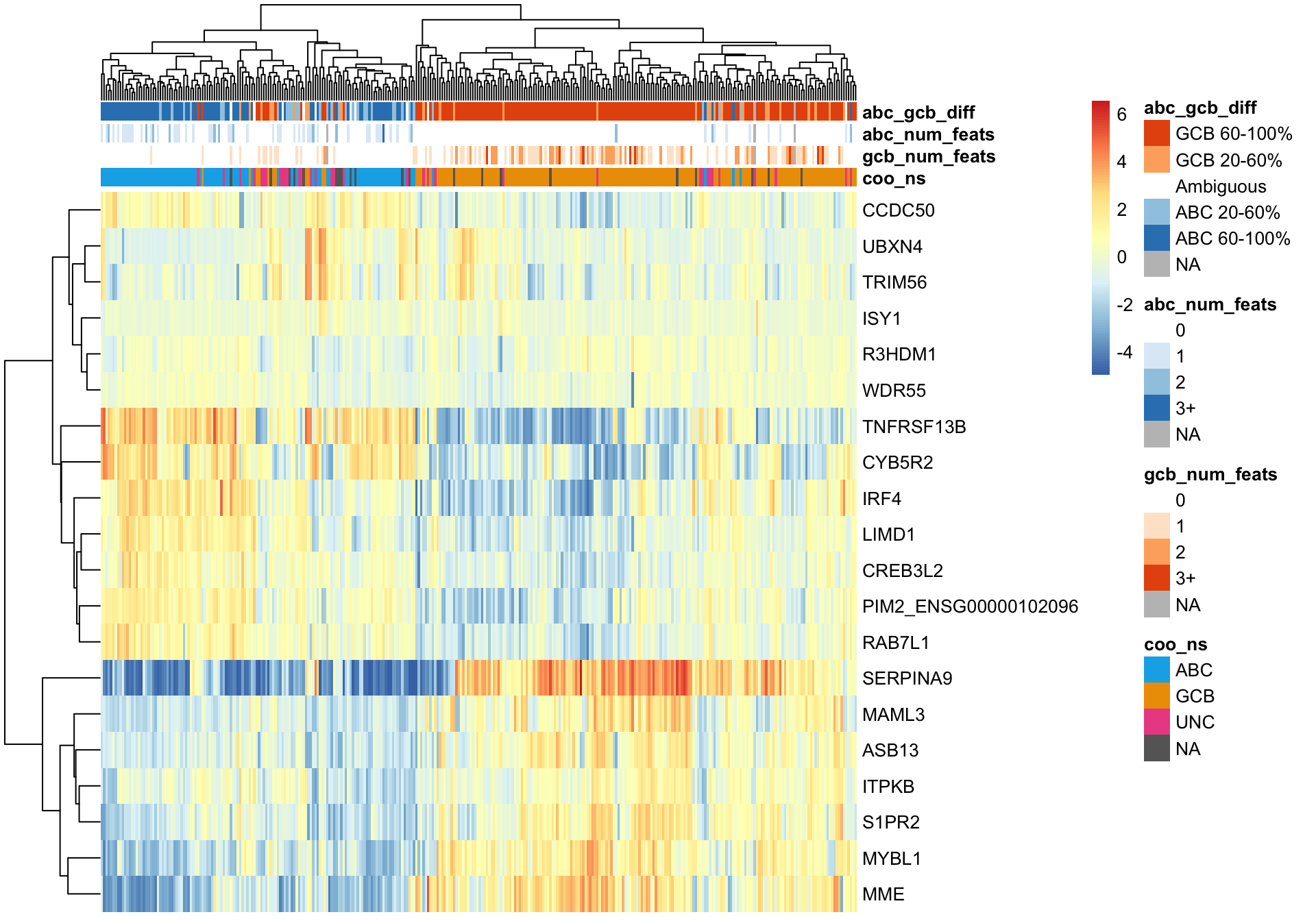
NF-κB Genes
texpr_nfkb <- texpr[gene_ids_filt %in% gene_ids$nfkb, ]
plot_heatmap(texpr_nfkb, coo_annot_mut_nmf, annotation_colors = colours)
Gene Set Enrichment Analysis
entrez_top_mad <-
  genes_df_filt %>%
  dplyr::slice(top_mad) %$%
  entrez %>%
  purrr::discard(~is.na(.x))