Data Loading and Tidying
Bruno Grande
2017-02-23 19:28:58
Metadata
Sample metadata
date_types <- readr::cols(lib_date = "c", seq_date = "c")

metadata         <- list()
metadata$patient <- read_tsv_quiet(paths$patient_md)
metadata$mrna    <- read_tsv_quiet(paths$mrna_md, col_types = date_types)

# Append TSS information to mRNA metadata
metadata$mrna <-
  metadata$patient %>%
  dplyr::select(patient, site, clinical_variant) %>%
  dplyr::left_join(metadata$mrna, ., by = "patient")
There happens to be a few patients with more than one RNA-seq dataset because both the FF and FFPE tumor tissue underwent library construction and sequencing. For now, we’ll simply be excluding the FFPE samples when an FF sample is available for the same patient.
metadata$mrna %<>%
  dplyr::group_by(patient) %>%
  dplyr::mutate(num_ff = sum(ff_or_ffpe == "FF")) %>%
  dplyr::filter(xor(num_ff > 0, ff_or_ffpe == "FFPE")) %>%
  dplyr::ungroup() %>%
  dplyr::select(-num_ff)
Gene/transcript metadata
tx2gene <- read_tsv_quiet(paths$tx2gene, col_names = c("transcript", "gene_id", "gene"))Results
Sex and EBV Status
We inferred sex and EBV status from the sequencing data because the clinical annotations were incomplete.
status <- list()

status$sex <-
  read_tsv_quiet(paths$sex_status) %>%
  dplyr::mutate(patient = get_patient_id(sample)) %>%
  dplyr::select(-sample, -chrY_chrX_read_ratio)

status$ebv <-
  read_tsv_quiet(paths$ebv_status) %>%
  dplyr::mutate(patient = get_patient_id(sample)) %>%
  dplyr::select(-sample, -ebv_read_ratio)

# Check if inferred sex status is consistent with incomplete clinical annotations
is_sex_consistent <-
  metadata$patient %>%
  dplyr::inner_join(status$sex, by = "patient") %$%
  ifelse(!is.na(annotated_sex), annotated_sex == sex, TRUE)
testthat::expect_true(all(is_sex_consistent))

# Fill in any blanks using the clinical annotations (e.g., the centroblast donors)
status$sex <-
  metadata$patient %>%
  dplyr::left_join(status$sex, by = "patient") %>%
  dplyr::mutate(sex = ifelse(is.na(sex), annotated_sex, sex)) %>%
  dplyr::select(patient, sex)

status$ebv <-
  metadata$patient %>%
  dplyr::left_join(status$ebv, by = "patient") %>%
  dplyr::mutate(
    ebv_status = ifelse(clinical_variant == "Centroblast", "Negative", ebv_status)) %>%
  dplyr::select(patient, ebv_status)

metadata <- purrr::map(metadata, ~dplyr::left_join(.x, status$sex, by = "patient"))
metadata <- purrr::map(metadata, ~dplyr::left_join(.x, status$ebv, by = "patient"))

rm(status)
Annotations
Now that the sex and EBV status are incorporated into the metadata data frames, we can create an annotations data frame. This is useful for certain tools like DEseq2 and pheatmap.
annotations <-
  metadata$mrna %>%
  dplyr::select(
    biospecimen_id, clinical_variant, ebv_status, sex,
    tissue_status, ff_or_ffpe, site, lib_date, seq_date) %>%
  dplyr::mutate_each(dplyr::funs(fill_na), -biospecimen_id) %>%
  dplyr::mutate_each("as.factor", -biospecimen_id) %>%
  as.data.frame() %>%
  tibble::column_to_rownames("biospecimen_id") %>%
  rev()
Legend Colours
Another thing we can do now that the metadata is loaded is define the legend colours.
colours <- get_legend_colours(metadata$mrna)

display_colours(colours, c(2, rep(3, length(colours)-1)))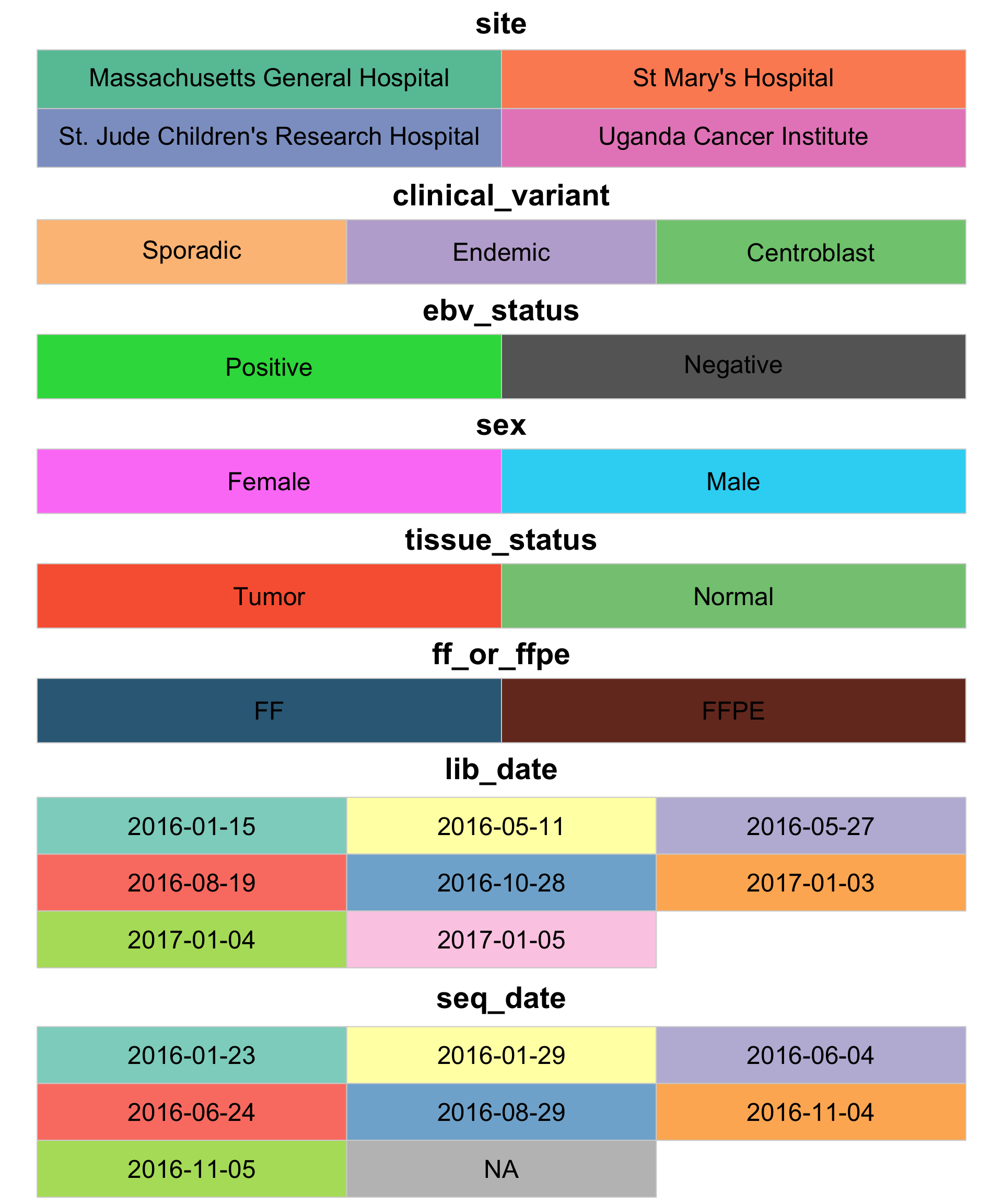
Salmon
We measured expression using Salmon (quasi-alignment). The transcriptome we used it Gencode v25 supplemented with EBV transcripts.
salmon             <- list()
salmon$txi         <- load_salmon(paths$salmon, tx2gene, metadata$mrna$biospecimen_id)
salmon$samples     <- colnames(salmon$txi$counts)
salmon$annotations <- annotations[salmon$samples,]