Exploring Salmon Results
Bruno Grande
2017-02-23
Raw Expression Counts
Lowly expressed genes
First, let’s observe the distribution of the median expression count per gene. Note that there is a long tail, and we’re just focusing on the small medians.
salmon_gene_stats <- get_stats(salmon$txi$counts, id_colname = "genes")

hist_salmon_gene_medians <-
  salmon_gene_stats %>% {
  ggplot(., aes(x = median)) +
  geom_histogram(binwidth = 1, fill = "grey75", colour = "grey40") +
  xlim(NA, quantile(.$median, 0.6))
}

hist_salmon_gene_medians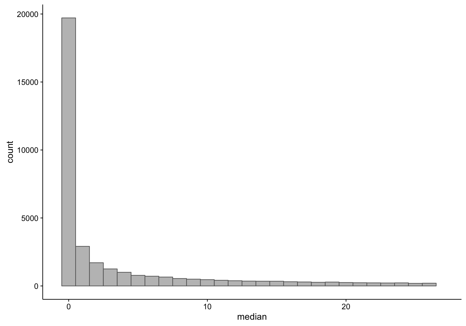
As you can see, there is a large proportion of genes whose expression medians are equal to zero: this affects 19418 out of 58133 genes. Just to make sure I’m not excluding genes that are highly expressed in less than half of the samples (but undetectable in the majority), I plot the average expression of these median-zero genes below.
hist_salmon_gene_means <-
  salmon_gene_stats %>%
  dplyr::filter(median == 0) %>% {
  ggplot(., aes(x = mean)) +
  geom_histogram(bins = 30, fill = "grey75", colour = "grey40") +
  xlim(NA, 5)
}

hist_salmon_gene_means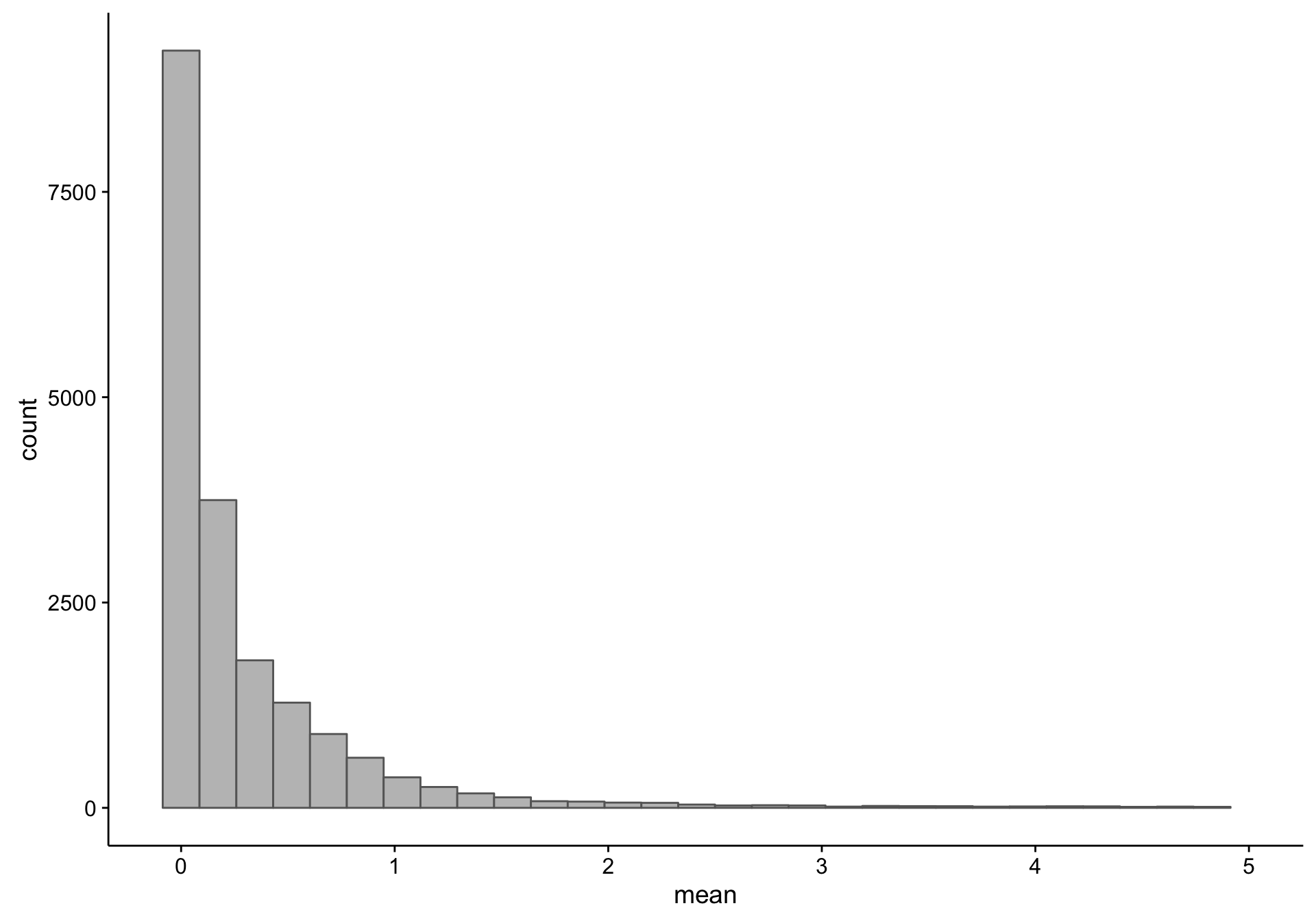
As you can see above, the average expression of these median-zero genes is extremely low for the vast majority: only 333 out of 19418 genes have an average expression count above five. Let’s plot the expressed of these genes to see whether it’s worth rescuing them, i.e. including them despite their median-zero status. Note that I’m scaling the values in each row.
median_zero_high_mean_genes <-
  hist_salmon_gene_means$data %>%
  dplyr::filter(mean > 5) %$%
  salmon$txi$counts[genes,]

plot_heatmap(median_zero_high_mean_genes, annotations, colours, border_color = NA)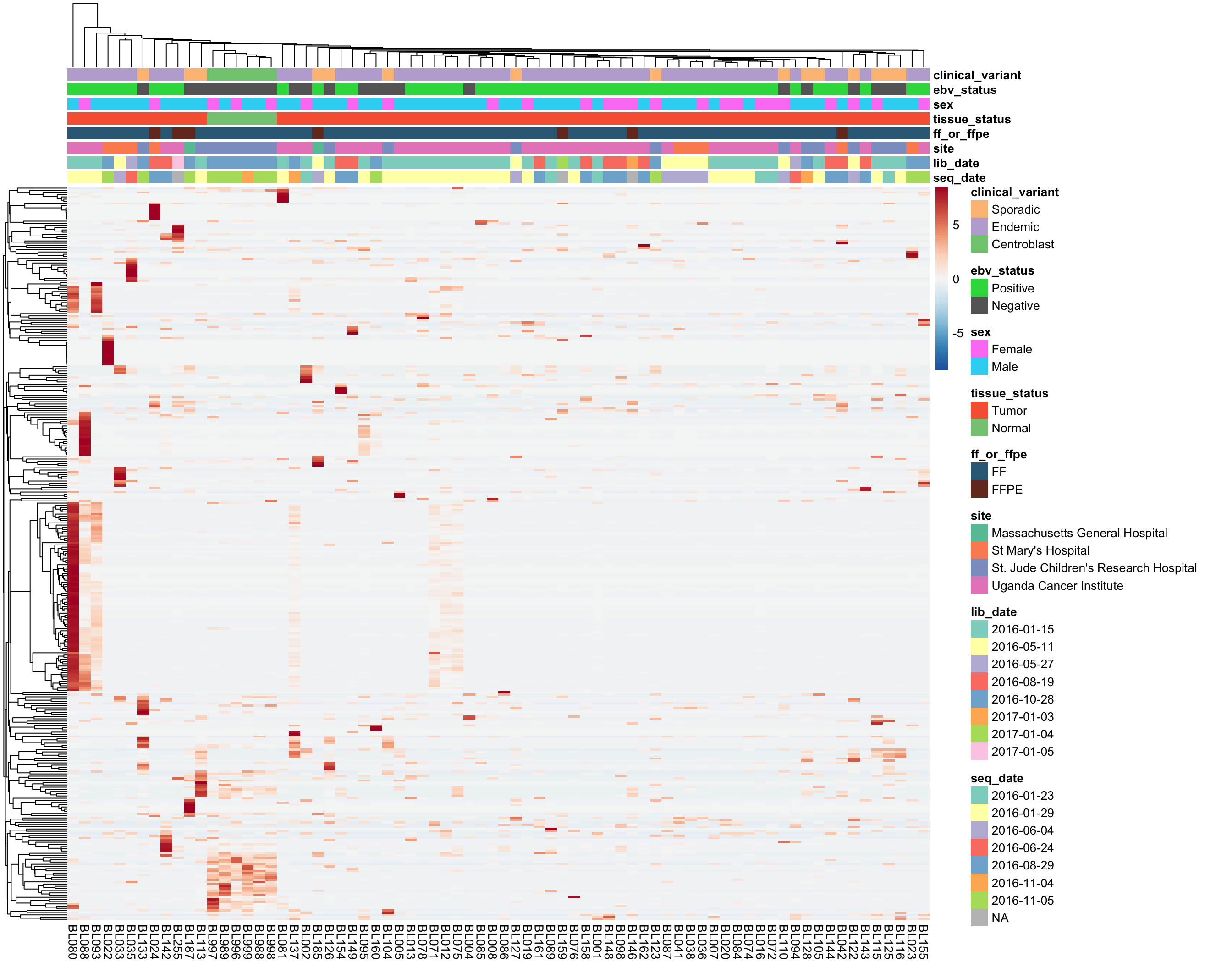
Based on the above heatmap, there doesn’t seem to be genes that are consistently expressed in less than half of the samples. Most genes seems to be highly expressed in a small subset of samples, most likely outliers. For this reason, these genes will not be rescued. I will now remove all median-zero genes.
mz_genes       <- salmon_gene_stats$median == 0
salmon$dds     <- DESeq2::DESeqDataSetFromTximport(
                     salmon$txi, salmon$annotations, ~tissue_status)
salmon$vst     <- DESeq2::vst(salmon$dds[!mz_genes,], blind = TRUE)
salmon$vst_mat <- SummarizedExperiment::assay(salmon$vst)
Transformed Expression Counts
Outlier samples
Now that we’ve removed uninformative genes, we should identify any outlier samples that should be excluded from downstream analyses. We will first look at the distribution of gene expression values. Note that we are using transformed (variance-stabilized) expression values.
scatterplot_salmon_sample_means_df <-
  salmon$vst_mat %>%
  t() %>%
  as.data.frame() %>%
  tibble::rownames_to_column("sample") %>%
  tidyr::gather(gene, expr, -sample)

scatterplot_salmon_sample_means_xorder <-
  scatterplot_salmon_sample_means_df %>%
  dplyr::group_by(sample) %>%
  dplyr::summarise(median = median(expr)) %>%
  dplyr::arrange(desc(median)) %$%
  sample

scatterplot_salmon_sample_means <-
  scatterplot_salmon_sample_means_df %>%
  ggplot(aes(x = sample, y = expr)) +
  geom_boxplot(fill = "grey75", colour = "grey40") +
  scale_x_discrete(limits = scatterplot_salmon_sample_means_xorder, labels = NULL)

scatterplot_salmon_sample_means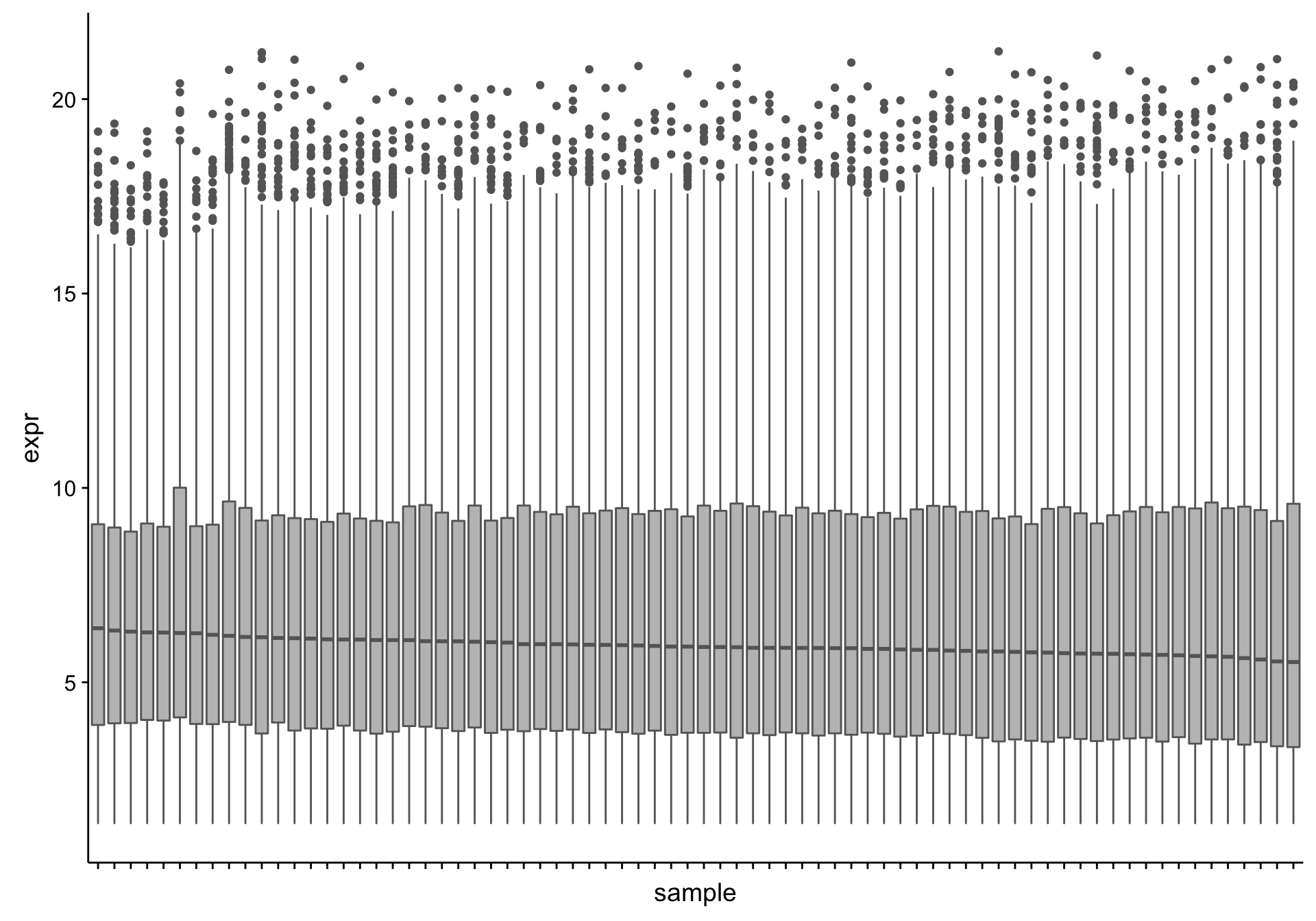
From the boxplots shown above, there doesn’t seem to be extreme outliers in terms of the median expression values. To check if there is an association between the median expression and any of the annotations we have for the RNA-seq samples, we plot a heatmap of the medians with covariate tracks.
salmon_sample_stats <- get_stats(salmon$vst_mat, id_colname = "biospecimen_id", transpose = TRUE)

salmon$vst_mat[, scatterplot_salmon_sample_means_xorder] %>%
  matrixStats::colMedians() %>%
  matrix(nrow = 1) %>%
  set_colnames(scatterplot_salmon_sample_means_xorder) %>%
  plot_heatmap(annotations, colours, cluster_rows = FALSE, cluster_cols = FALSE)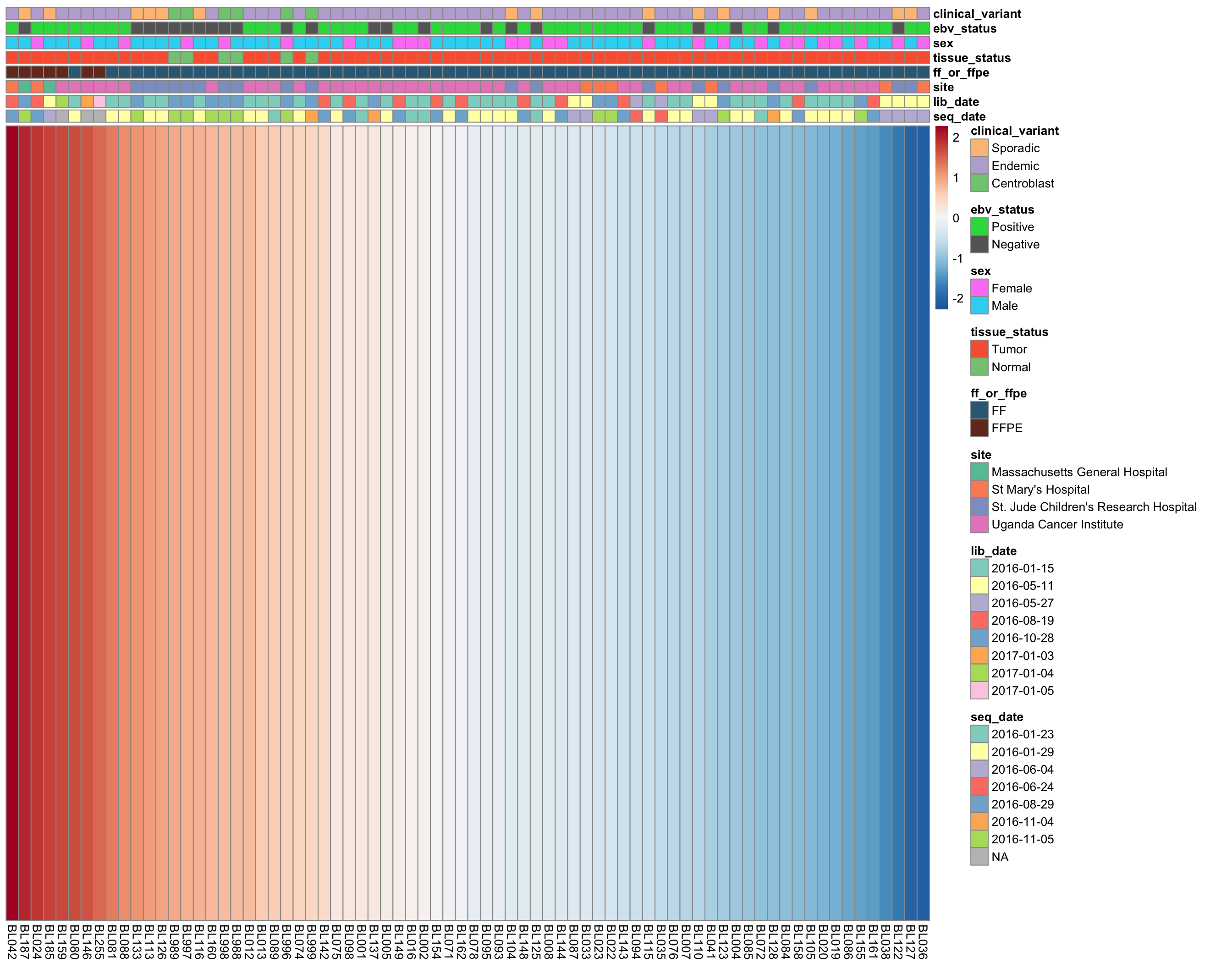
wilcox_median_ff_or_ffpe <-
  salmon_sample_stats %>%
  dplyr::left_join(metadata$mrna, by = "biospecimen_id") %$%
  wilcox.test(median[ff_or_ffpe == "FF"], median[ff_or_ffpe == "FFPE"])
Strikingly, the samples with the highest median expressed are significantly enriched in FFPE samples (p = 1.8310^{-5}, Mann-Whitney-U test). It’s not yet clear whether this is ground for omitting the FFPE samples. We will wait until we see the results from unsupervised clustering below.
Principle component analysis
The first approach to unsupervised clustering is a principle component analysis. This will identify is the major sources of variation (_e.g._PC1, PC2) are explained by technical or biological features.
pca <- calc_pca(salmon$vst)

pca_plots <-
  names(annotations) %>%
  purrr::map(~plot_pca(pca, .x, colours, c(1,1)))

gridExtra::grid.arrange(grobs = pca_plots, ncol = 3)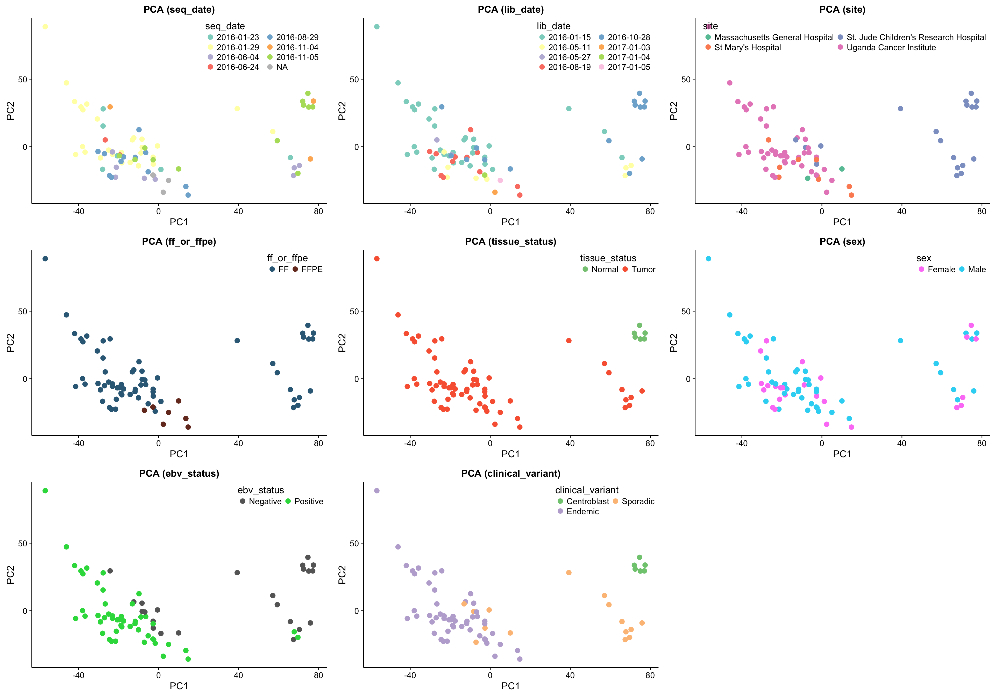
The above set of PCA plots are reassuring for the following reasons:
- There doesn’t seem to be clear clustering according to technical features such as library or sequencing date.
- The normal samples (centroblasts) cluster together, suggesting little variability in the centroblast expression profiles.
- The FFPE samples, while they still cluster together, do not significantly separate themselves from the remaining tumour samples.
Focusing on the tumour samples, there are two clear clusters: a big one and a smaller one. None of the features perfectly account for the separation of the small cluster from the big cluster. Some features come close though and warrant further investigation (e.g. site, EBV status and clinical variant status).
As a sanity check, the scree plot corresponding to the above PCA is shown below.
screeplot_salmon <-
  pca$percent_var %>%
  dplyr::slice(1:10) %>%
  ggplot(aes(x = pc, y = percent_var, group = "all")) +
  geom_point() +
  geom_line()

screeplot_salmon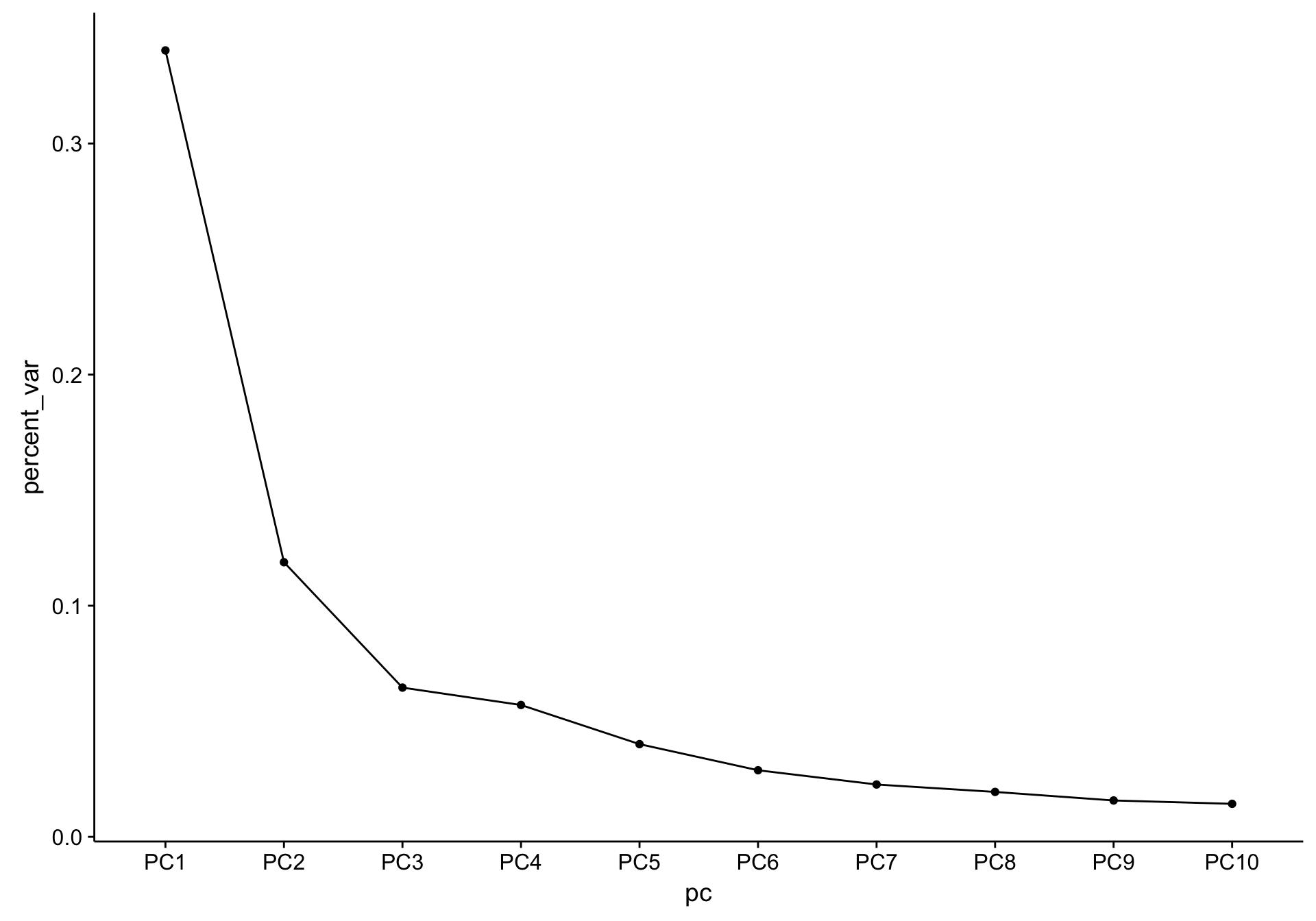
There is a substantial difference between the variance explained by PC1 and PC2, but nothing worrisome.
Hierarchical clustering
most_var <- subset_most_variable_genes(salmon$vst_mat, 1000)

heatmap_salmon_most_var <- plot_heatmap(most_var, annotations, colours)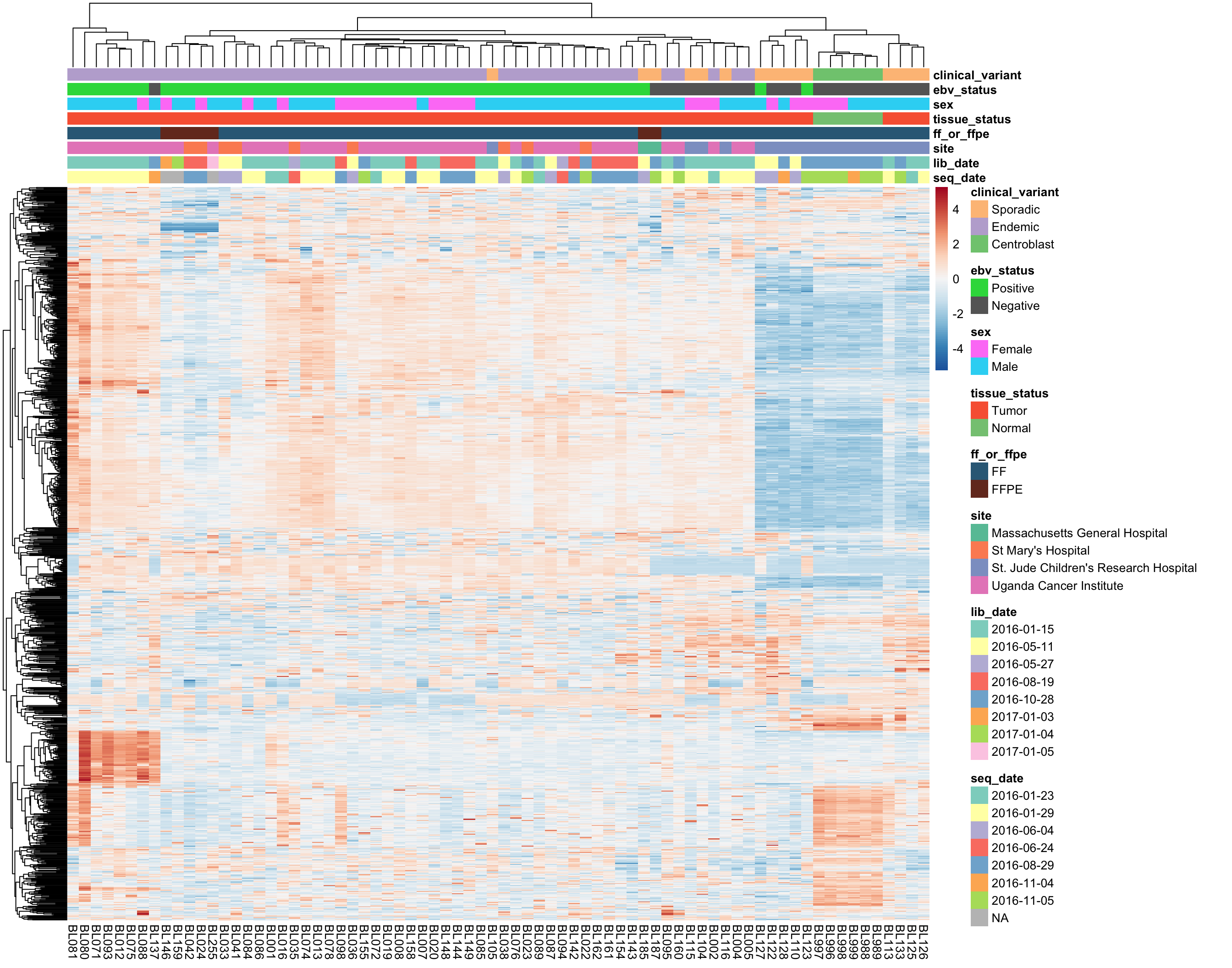
The above heatmap highlights a clear sample outgroup defined by high expressed of a subset of genes.
Consensus Clustering
ccp <- ConsensusClusterPlus::ConsensusClusterPlus(
  salmon$vst_mat, maxK = 5, pItem = 0.8, pFeature = 0.8, seed = global_seed)