Predicting COO Using Mutation Data
Bruno Grande
2017-02-14 00:16:57
Before exploring the expression data, I want to obtain a list of mutation features that help predict COO. Here, I define mutation features as being a mutated hotspot or gene. This information will help evaluate downstream clustering solutions.
Two methods will be compared below. Both will be using the Lymphp2Cx COO labels as an approximation of ground truth. The first approach will use Fisher’s exact test to identify mutation features that are significantly associated with COO. The second approach will leverage a random forest model to rank the importance of mutation features.
Identifying Mutation Hotspots
Before ranking mutation features, we need to identify mutation hotspots, because some are known to be associated with COO (e.g. MYD88 and EZH2 hotspot mutations). For this, we are identifying recurrently altered codons, i.e. those that are present in at least 5% of patients.
hotspots <-
  muts %>%
  dplyr::group_by(gene, codon) %>%
  dplyr::mutate(num_affected = dplyr::n_distinct(patient),
                hotspot = num_affected > length(patients$rnaseq) * min_recur,
                hotspot = ifelse(type != "missense", FALSE, hotspot),
                feature = ifelse(hotspot, paste0(gene, "_", codon), paste0(gene, "_other"))) %>%
  dplyr::ungroup()


mut_features <-
  hotspots %>%
  dplyr::select(patient, feature) %>%
  dplyr::distinct() %>%
  tidyr::spread(patient, patient) %>%
  tidyr::gather(patient, status, -feature) %>%
  dplyr::mutate(mutated = !is.na(status),
                status = NULL) %>%
  dplyr::left_join(coo, by = "patient")

heatmap_mut_annot <-
  coo %>%
  dplyr::filter(coo_ns %in% c("ABC", "GCB"),
                patient %in% mut_features$patient) %>%
  tibble::column_to_rownames("patient")

mut_feat_df <-
  mut_features %>%
  dplyr::mutate(mutated = ifelse(mutated, 1, 0)) %>%
  tidyr::spread(feature, mutated)

mut_feat_matrix_all <-
  mut_feat_df %>%
  dplyr::select(-coo_ns) %>%
  as.data.frame() %>%
  set_rownames(c()) %>%
  tibble::column_to_rownames("patient") %>%
  as.matrix() %>%
  t() %>%
  extract(, order(coo %>% dplyr::filter(patient %in% mut_features$patient) %$% coo_ns))

mut_feat_matrix <-
  mut_feat_matrix_all %>%
  extract(, colnames(.) %in% rownames(heatmap_mut_annot))

hotspots %>%
  dplyr::filter(hotspot) %>%
  dplyr::select(gene, codon, num_affected) %>%
  dplyr::distinct() %>%
  dplyr::arrange(desc(num_affected)) %>%
knitr::kable(caption = "Recurrently altered gene codons (hotspots)")| gene | codon | num_affected |
|---|---|---|
| EZH2 | 646 | 41 |
| MYD88 | 273 | 35 |
| B2M | 1 | 28 |
| CD79B | 197 | 20 |
| MEF2B | 83 | 19 |
Ranking Mutation Features
Approach #1: Fisher’s exact test
A simple approach to ranking mutation features is to statistically test for an association between a feature and COO status. Because this is count data, the Fisher’s exact test can be used. After performing BH multiple test correction, we filter for features with a minimum q-value of 10%.
mut_fisher <-
  mut_features %>%
  dplyr::filter(coo_ns %in% c("ABC", "GCB")) %>%
  dplyr::group_by(feature) %>%
  tidyr::nest() %>%
  dplyr::mutate(fisher = purrr::map(data, ~fisher.test(.$mutated, .$coo_ns)),
                p_val = purrr::map_dbl(fisher, "p.value"),
                q_val = p.adjust(p_val, method = p_adjust_method)) %>%
  dplyr::select(-data, -fisher) %>%
  dplyr::arrange(q_val) %>%
  dplyr::filter(q_val < qval_cutoff)

knitr::kable(mut_fisher)| feature | p_val | q_val |
|---|---|---|
| TNFRSF14_other | 0.0000000 | 0.0000000 |
| GNA13_other | 0.0000000 | 0.0000000 |
| MYD88_273 | 0.0000000 | 0.0000000 |
| NFKBIZ_other | 0.0000010 | 0.0000207 |
| CD79B_197 | 0.0000031 | 0.0000451 |
| EZH2_646 | 0.0000029 | 0.0000451 |
| CREBBP_other | 0.0000050 | 0.0000617 |
| BCL2_other | 0.0000067 | 0.0000720 |
| SOCS1_other | 0.0000209 | 0.0001999 |
| P2RY8_other | 0.0000429 | 0.0003691 |
| PIM1_other | 0.0000656 | 0.0005127 |
| MPEG1_other | 0.0001752 | 0.0012555 |
| MEF2B_83 | 0.0004585 | 0.0030332 |
| TMSB4X_other | 0.0005130 | 0.0031516 |
| SGK1_other | 0.0007329 | 0.0042018 |
| USP7_other | 0.0008055 | 0.0043293 |
| TBL1XR1_other | 0.0035960 | 0.0181914 |
| IL4R_other | 0.0073326 | 0.0350336 |
| IRF8_other | 0.0081798 | 0.0370245 |
| CD79B_other | 0.0088917 | 0.0382342 |
| BCL10_other | 0.0229202 | 0.0938636 |
heatmap_mut_fisher <-
  mut_feat_matrix %>%
  extract(mut_fisher$feature, ) %>%
  pheatmap::pheatmap(cluster_rows = FALSE, cluster_cols = FALSE, show_colnames = FALSE,
                     color = colours$mutated, legend = FALSE,
                     annotation_col = heatmap_mut_annot,
                     annotation_colors = colours,
                     gaps_col = sum(heatmap_mut_annot$coo_ns == "ABC"))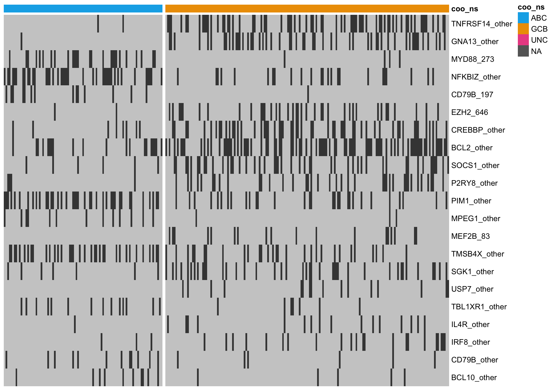
Approach #2: Random forest
Mutation features can also be ranked using machine learning. Here, we are training a random forest model to predict COO from the mutation features. A side-product from training this model is the feature importance, which we can use as a ranking.
# Remove any features with near-zero variance
nz_feats <- caret::nearZeroVar(mut_feat_df)
abc_gcb_rows <- mut_feat_df$coo_ns %in% c("ABC", "GCB")
mut_rf_patients <- mut_feat_df[abc_gcb_rows, 1]
mut_feat_df_no_nz <- mut_feat_df[abc_gcb_rows, -c(1, nz_feats)]

mut_ctrl <- caret::trainControl(method = "cv", number = 10)

mut_model <-
  caret::train(coo_ns ~ ., mut_feat_df_no_nz, method = "rf",
               preProcess = "scale", trControl = mut_ctrl, tuneLength = 10)
mut_model
Random Forest
265 samples
63 predictor
2 classes: 'ABC', 'GCB'
Pre-processing: scaled (63)
Resampling: Cross-Validated (10 fold)
Summary of sample sizes: 239, 238, 239, 239, 239, 238, ...
Resampling results across tuning parameters:
mtry Accuracy Kappa
2 0.8183761 0.5766302
8 0.8525641 0.6766409
15 0.8562678 0.6835703
22 0.8411681 0.6516932
29 0.8450142 0.6598058
35 0.8525641 0.6766336
42 0.8411681 0.6519934
49 0.8299145 0.6261980
56 0.8376068 0.6454647
63 0.8336182 0.6333382
Accuracy was used to select the optimal model using the largest value.
The final value used for the model was mtry = 15. mut_imp <- caret::varImp(mut_model, scale = FALSE)
mut_rf <-
mut_imp$importance %>%
tibble::rownames_to_column("feature") %>%
dplyr::rename(importance = Overall) %>%
dplyr::arrange(desc(importance)) %>%
head(nrow(mut_fisher))
knitr::kable(mut_rf)| feature | importance |
|---|---|
| TNFRSF14_other | 12.067403 |
| MYD88_273 | 10.101535 |
| GNA13_other | 7.666659 |
| NFKBIZ_other | 6.964802 |
| BCL2_other | 4.487544 |
| CREBBP_other | 4.305662 |
| P2RY8_other | 3.908851 |
| SOCS1_other | 3.728200 |
| CD79B_197 | 3.564910 |
| SGK1_other | 3.164051 |
| TMSB4X_other | 2.860404 |
| EZH2_646 | 2.806504 |
| PIM1_other | 2.642619 |
| MPEG1_other | 1.856701 |
| GABRB3_other | 1.845886 |
| KMT2D_other | 1.730061 |
| B2M_1 | 1.619111 |
| TP53_other | 1.567689 |
| KMT2C_other | 1.509390 |
| TMEM30A_other | 1.476182 |
| IRF4_other | 1.423674 |
heatmap_mut_rf <-
  mut_feat_matrix %>%
  extract(mut_rf$feature, ) %>%
  pheatmap::pheatmap(cluster_rows = FALSE, cluster_cols = FALSE, show_colnames = FALSE,
                     color = colours$mutated, legend = FALSE,
                     annotation_col = heatmap_mut_annot,
                     annotation_colors = colours,
                     gaps_col = sum(heatmap_mut_annot$coo_ns == "ABC"))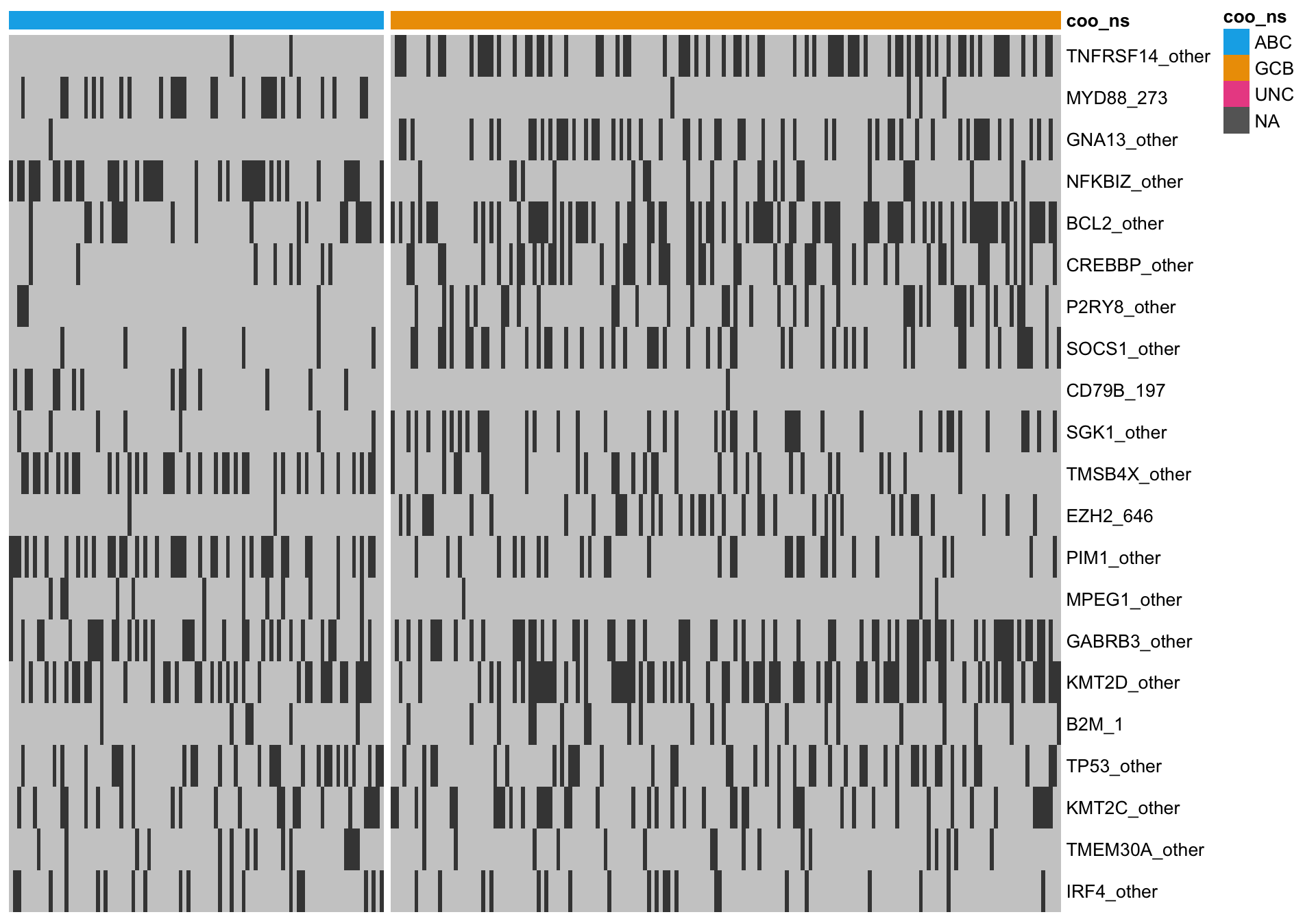
Hybrid approach
Unsurprisingly, both approaches share several highly ranked features. A hybrid approach here considers the overlap between both methods, which should select the most informative genes.
All overlapping genes
When I consider the overlap, there are several genes that visually do not seem to discriminate well between ABC and GCB cases. One issue is that we are using the Lymph2Cx labels, which we guess are not perfect. Therefore, some cases might be on the right side of the heatmap, so to speak.
mut_hybrid_df <-
  mut_feat_df %>%
  tidyr::gather(feature, mutated, -patient, -coo_ns) %>%
  dplyr::filter(feature %in% intersect(mut_fisher$feature, mut_rf$feature)) %>%
  dplyr::group_by(feature, coo_ns) %>%
  dplyr::summarise(num_mutated = sum(mutated)) %>%
  tidyr::spread(coo_ns, num_mutated) %>%
  dplyr::mutate(ratio = ABC / GCB) %>%
  dplyr::arrange(ratio)

mut_hybrid_all <- mut_hybrid_df$feature

heatmap_mut_hybrid <-
  mut_feat_matrix %>%
  extract(mut_hybrid_all, ) %>%
  pheatmap::pheatmap(cluster_rows = FALSE, cluster_cols = FALSE, show_colnames = FALSE,
                     color = colours$mutated, legend = FALSE,
                     annotation_col = heatmap_mut_annot,
                     annotation_colors = colours,
                     gaps_col = sum(heatmap_mut_annot$coo_ns == "ABC"))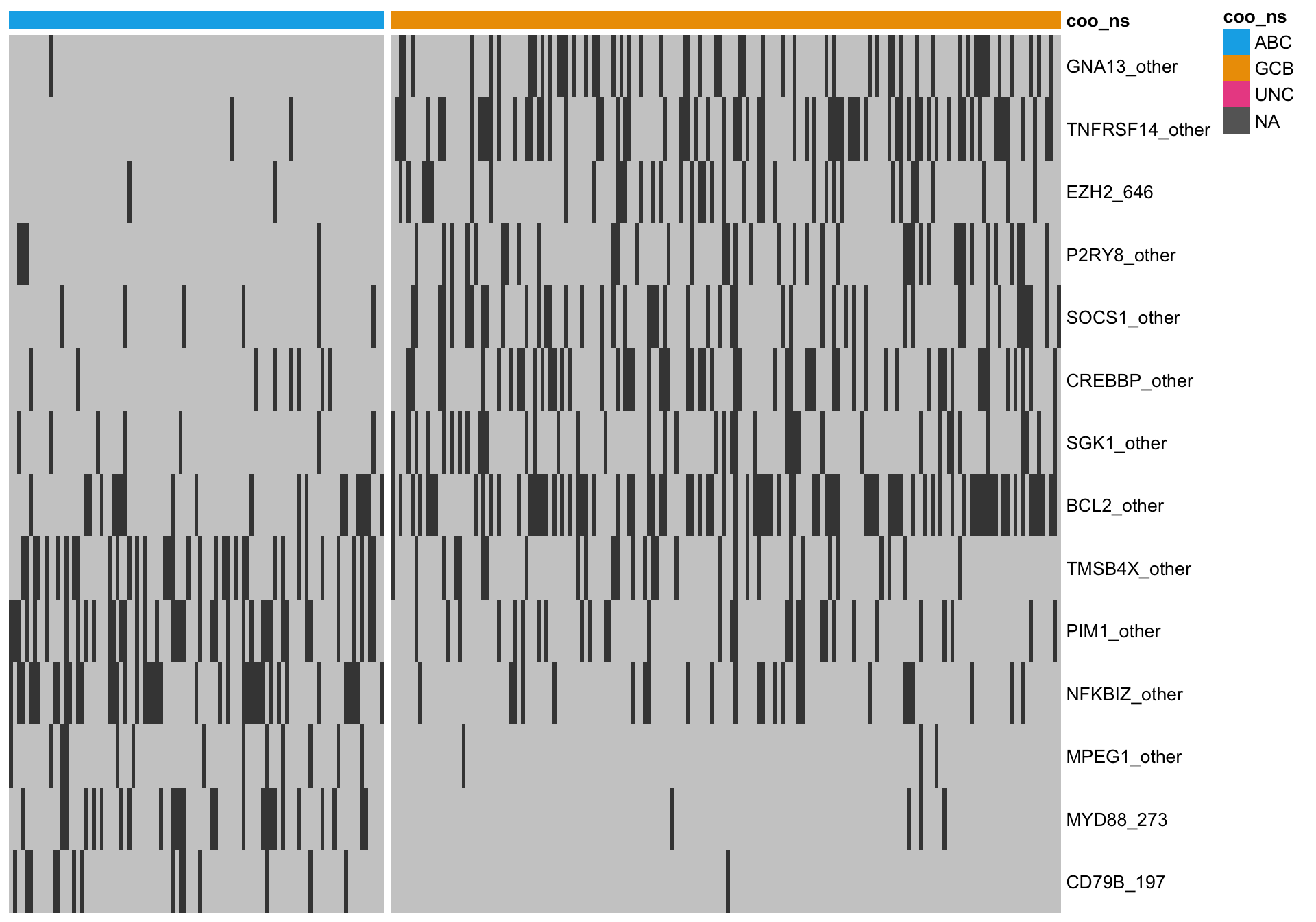
Most discriminating genes
Here, I’m only considering genes with the most extreme ratio of ABC-mutated cases versus GCB-mutated cases. This set of more amenable to simple counting of the number of ABC/GCB-associated mutation features.
mut_hybrid_df_top <-
  mut_hybrid_df %>%
  dplyr::filter(ratio < 0.1 | ratio > 2)

heatmap_mut_hybrid_top <-
  mut_feat_matrix %>%
  extract(mut_hybrid_df_top$feature, ) %>%
  pheatmap::pheatmap(cluster_rows = FALSE, cluster_cols = FALSE, show_colnames = FALSE,
                     color = colours$mutated, legend = FALSE,
                     annotation_col = heatmap_mut_annot,
                     annotation_colors = colours,
                     gaps_col = sum(heatmap_mut_annot$coo_ns == "ABC"))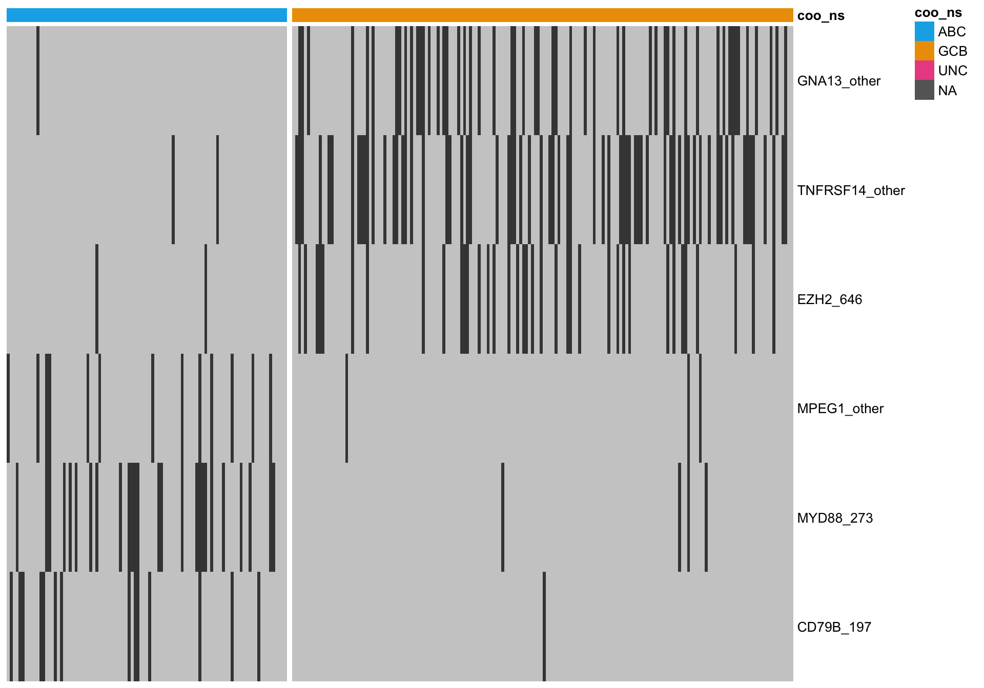
Predicting COO
Counting discriminating features
gcb_features <- mut_hybrid_df_top %>% dplyr::filter(ratio < 1) %$% feature
abc_features <- mut_hybrid_df_top %>% dplyr::filter(ratio > 1) %$% feature

discretize <- function(x) {
  dplyr::recode(x, `0` = "0", `1` = "1", `2` = "2", .default = "3+")
}

num_feats <-
  mut_features %>%
  dplyr::filter(mutated) %>%
  dplyr::group_by(patient, coo_ns) %>%
  dplyr::summarise(gcb_num_feats = discretize(sum(feature %in% gcb_features)),
                   abc_num_feats = discretize(sum(feature %in% abc_features)))

heatmap_mut_hybrid_num_feats_annot <-
  num_feats %>%
  as.data.frame() %>%
  tibble::column_to_rownames("patient") %>%
  dplyr::ungroup()

barplot_mut_hybrid_num_feats <-
  heatmap_mut_hybrid_num_feats_annot %>%
  dplyr::select(-coo_ns,
                `Number of ABC features` = abc_num_feats,
                `Number of GCB features` = gcb_num_feats) %>%
  tidyr::gather(type, count) %>%
  dplyr::count(type, count) %>%
  ggplot(aes(x = count, y = n)) +
  geom_bar(stat = "identity") +
  facet_grid(~type) +
  labs(title = "Number of patients per mutation feature count",
       x = "Number of ABC/GCB features", y = "Number of patients")
barplot_mut_hybrid_num_feats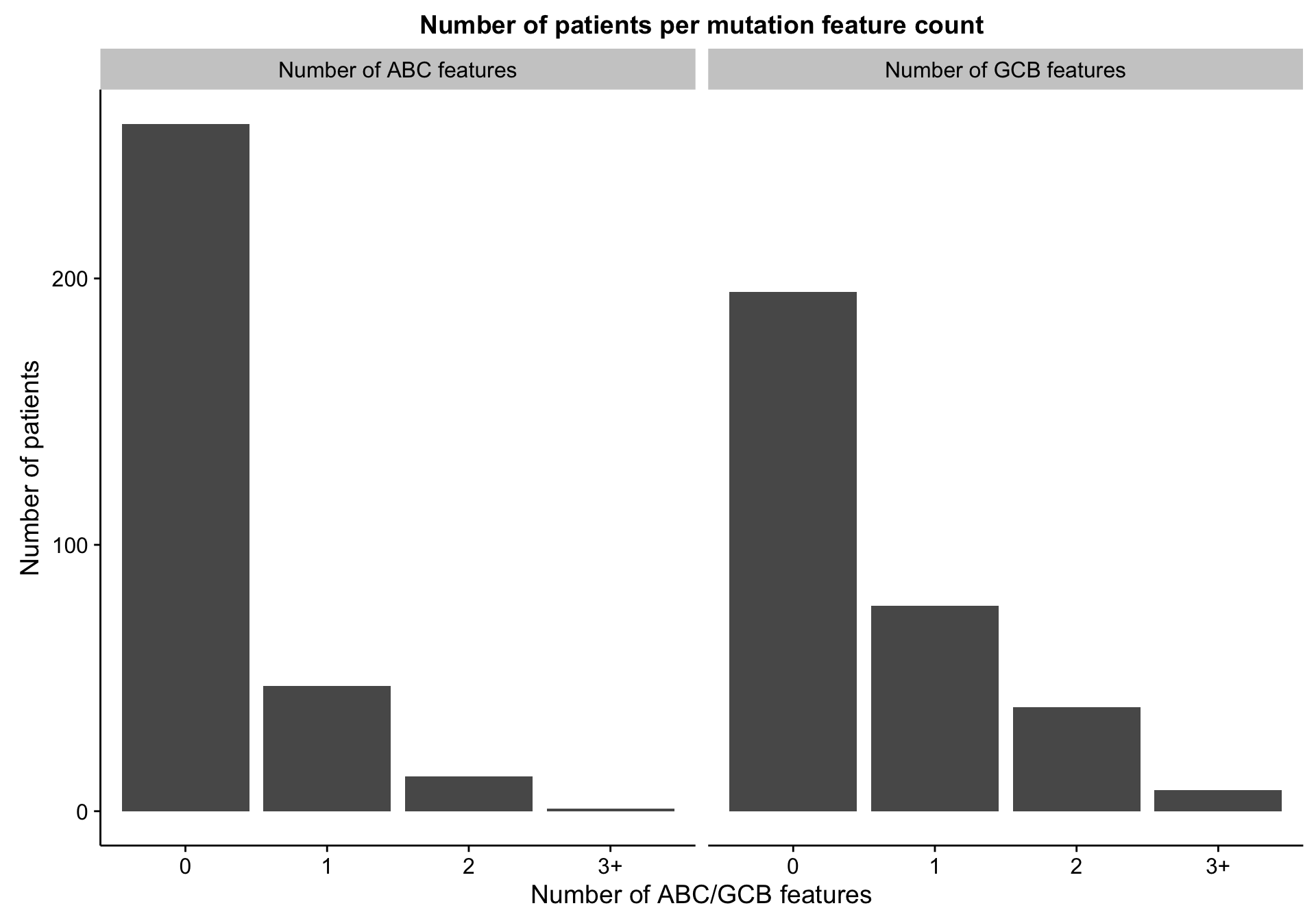
Random forest probability
# discretize_probs <- function(x) {
#   cut(x, breaks = c(0, 0.2, 0.4, 0.6, 0.8, 1),
#       labels = c("0-20%", "20-40%", "40-60%", "60-80%", "80-100%")) %>%
#     as.character()
# }

discretize_diff <- function(x) {
  cut(x, breaks = c(-1.1, -0.6, -0.2, 0.2, 0.6, 1.1),
      labels = c("GCB 60-100%", "GCB 20-60%", "Ambiguous", "ABC 20-60%", "ABC 60-100%")) %>%
    as.character()
}

# mut_rf_prob_df <-
#   predict(mut_model, mut_feat_df_no_nz, "prob") %>%
#   dplyr::transmute(abc_rf_prob = discretize_probs(ABC),
#                    gcb_rf_prob = discretize_probs(GCB)) %>%
#   dplyr::bind_cols(mut_rf_patients)

mut_rf_prob_df <-
  predict(mut_model, mut_feat_df, "prob") %>%
  dplyr::transmute(abc_gcb_diff = discretize_diff(ABC - GCB)) %>%
  dplyr::bind_cols(mut_feat_df[,"patient"])

heatmap_mut_rf_prob_annot <-
  heatmap_mut_hybrid_num_feats_annot %>%
  tibble::rownames_to_column("patient") %>%
  dplyr::left_join(mut_rf_prob_df) %>%
  tibble::column_to_rownames("patient") %>%
  extract(, c("coo_ns", "gcb_num_feats", "abc_num_feats", "abc_gcb_diff"))

barplot_mut_rf_prob_data <-
  heatmap_mut_rf_prob_annot %>%
  dplyr::select(-dplyr::ends_with("_num_feats"),
                `P(ABC) - P(GCB)` = abc_gcb_diff) %>%
  tidyr::gather(type, prob, -coo_ns) %>%
  dplyr::count(coo_ns, type, prob) %>%
  dplyr::mutate(prob = factor(prob, names(colours$abc_gcb_diff)[1:5]))

barplot_mut_rf_prob <-
  barplot_mut_rf_prob_data %>%
  ggplot(aes(x = prob, y = n, fill = coo_ns)) +
  geom_bar(stat = "identity") +
  scale_x_discrete(drop = FALSE) +
  scale_fill_manual(values = colours$coo_ns) +
  place_legend(c(1, 1)) +
  labs(title = "Number of patients per RF probability range",
       x = "P(ABC) - P(GCB)", y = "Number of patients", fill = "Lymph2Cx COO")
barplot_mut_rf_prob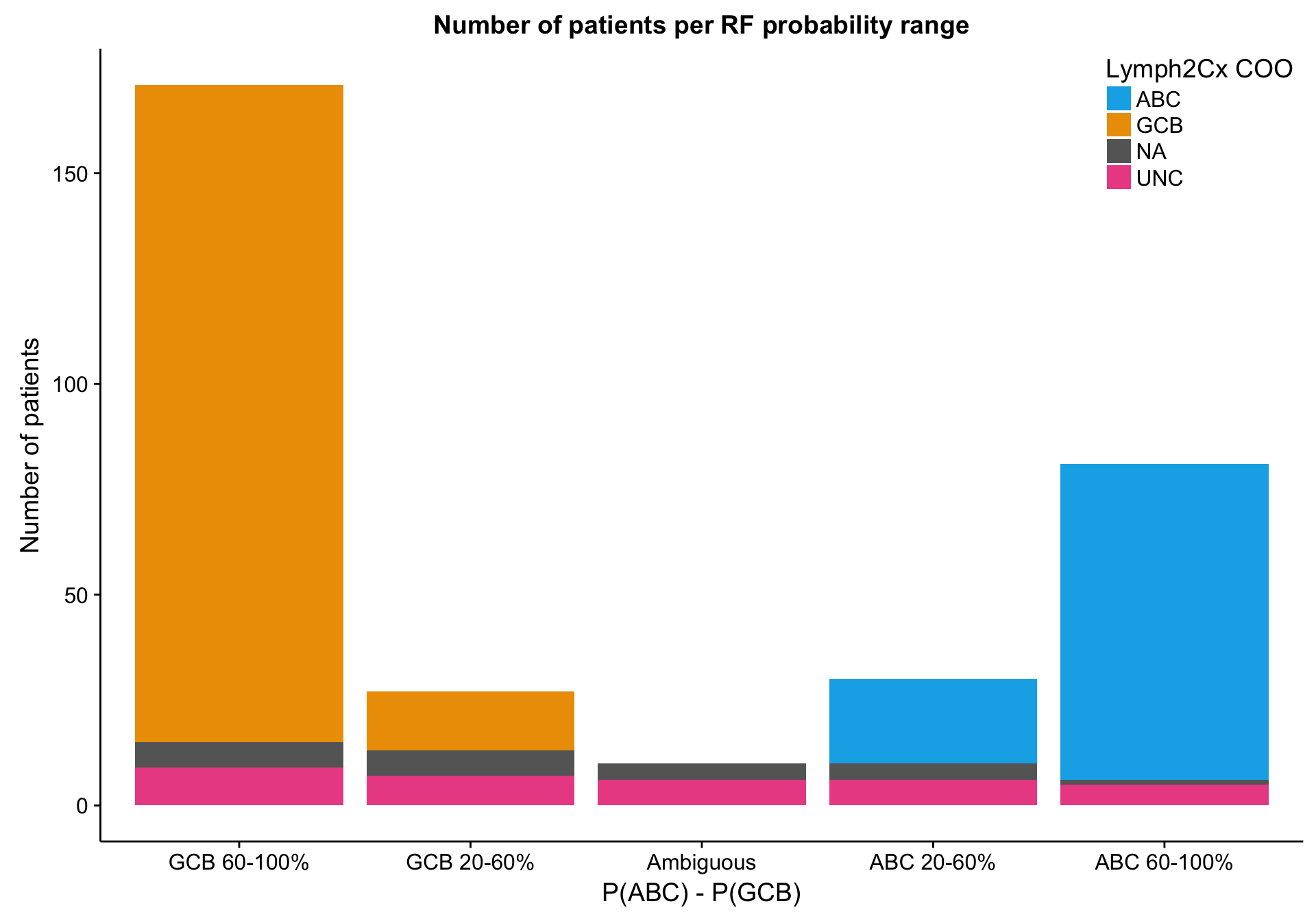
patient_no_mut <-
  mut_feat_df %>%
  dplyr::transmute(patient, total = rowSums(.[, -(1:2)])) %>%
  dplyr::filter(total < 5) %$%
  patient

heatmap_mut_rf_prob_annot_no_mut <-
  heatmap_mut_rf_prob_annot %>%
  tibble::rownames_to_column("patient") %>%
  dplyr::filter(patient %in% patient_no_mut) %>%
  dplyr::select(-dplyr::ends_with("_num_feats"),
                `P(ABC) - P(GCB)` = abc_gcb_diff,
                -patient) %>%
  tidyr::gather(type, prob, -coo_ns) %>%
  dplyr::count(coo_ns, type, prob) %>%
  dplyr::mutate(prob = factor(prob, names(colours$abc_gcb_diff)[1:5]))

barplot_mut_rf_prob_no_mut <-
  barplot_mut_rf_prob %+%
  heatmap_mut_rf_prob_annot_no_mut +
  labs(title = paste0(barplot_mut_rf_prob$labels$title, "\n(Patients with <5 mutations)")) +
  place_legend(c(0.5, 1))
barplot_mut_rf_prob_no_mut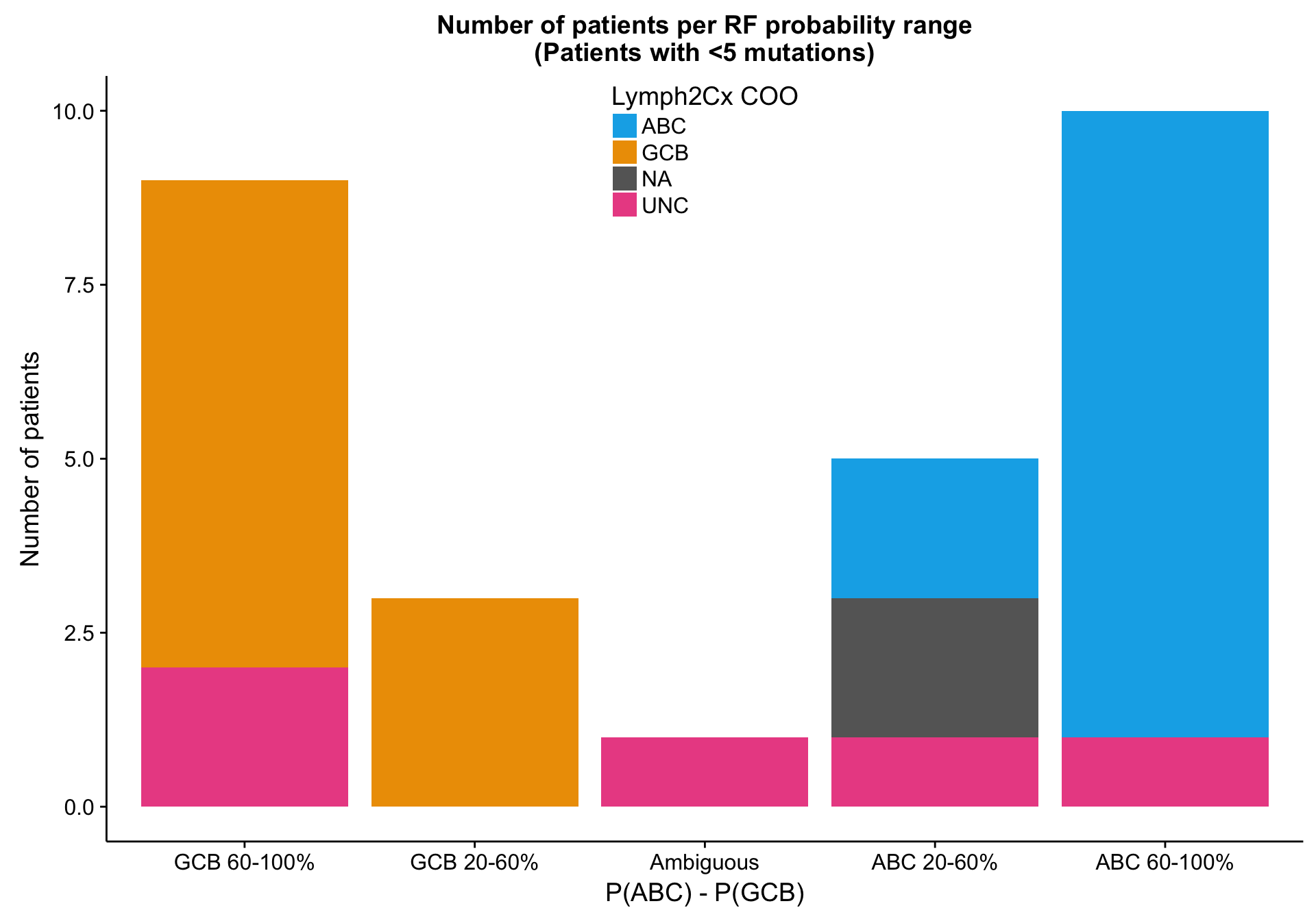
lineplot_mut_rf_prob_df <-
  predict(mut_model, mut_feat_df, "prob") %>%
  dplyr::bind_cols(mut_feat_df[,c("patient", "coo_ns")]) %>%
  tibble::rownames_to_column("id") %>%
  dplyr::ungroup() %>%
  dplyr::mutate(id = forcats::fct_reorder(id, ABC),
                prob = GCB)

scatterplot_rf_prob_vs_num_muts_df <-
  mut_feat_df %>%
  tidyr::gather(feature, num_muts, -patient, -coo_ns) %>%
  dplyr::group_by(patient) %>%
  dplyr::summarise(total_muts = sum(num_muts)) %>%
  dplyr::left_join(lineplot_mut_rf_prob_df, by = "patient")

scatterplot_rf_prob_vs_num_muts <-
  scatterplot_rf_prob_vs_num_muts_df %>% {
    ymax <- max(.$total_muts) + 2
    ggplot(., aes(x = GCB, y = total_muts, colour = coo_ns)) +
    annotate("rect", xmin = 0, xmax = 0.5, ymin = 0, ymax = ymax,
             fill = colours$coo["ABC"], alpha = 0.1) +
    annotate("rect", xmin = 0.5, xmax = 1, ymin = 0, ymax = ymax,
             fill = colours$coo["GCB"], alpha = 0.1) +
    geom_vline(xintercept = 0.5) +
    geom_point() +
    scale_x_continuous(limits = c(0, 1), expand = c(0, 0)) +
    scale_y_continuous(limits = c(0, ymax), expand = c(0, 0)) +
    scale_color_manual(values = colours$coo) +
    labs(title = paste0("Relationship between probability for GCB and number of mutations\n",
                        "(Background colour corresponds to random forest prediction)"),
           x = "Probability for GCB", y = "Number of mutations", colour = "Lymph2Cx COO") +
    place_legend(c(0, 1))
  }
scatterplot_rf_prob_vs_num_muts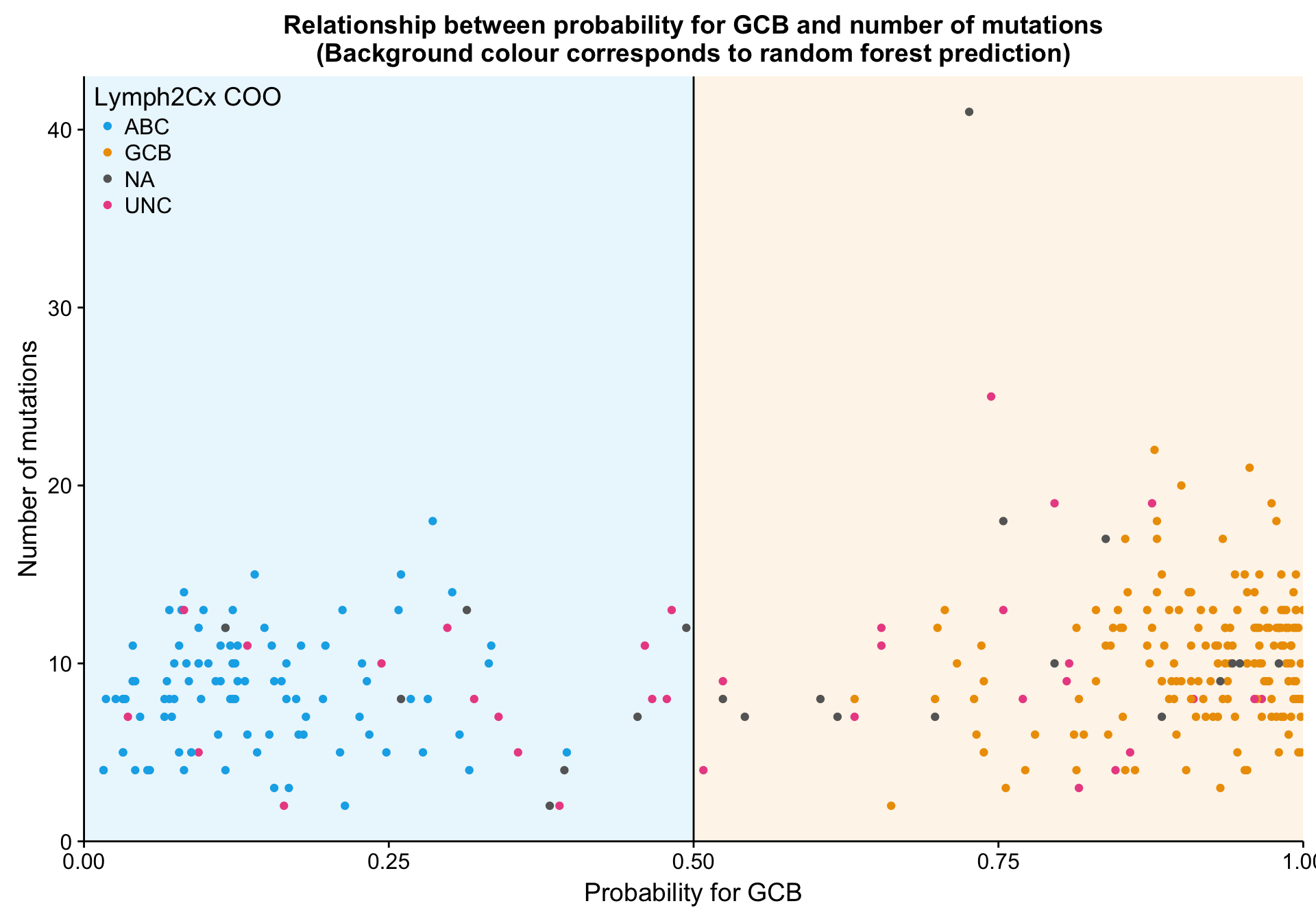
n_patients <- ncol(mut_feat_matrix_all)
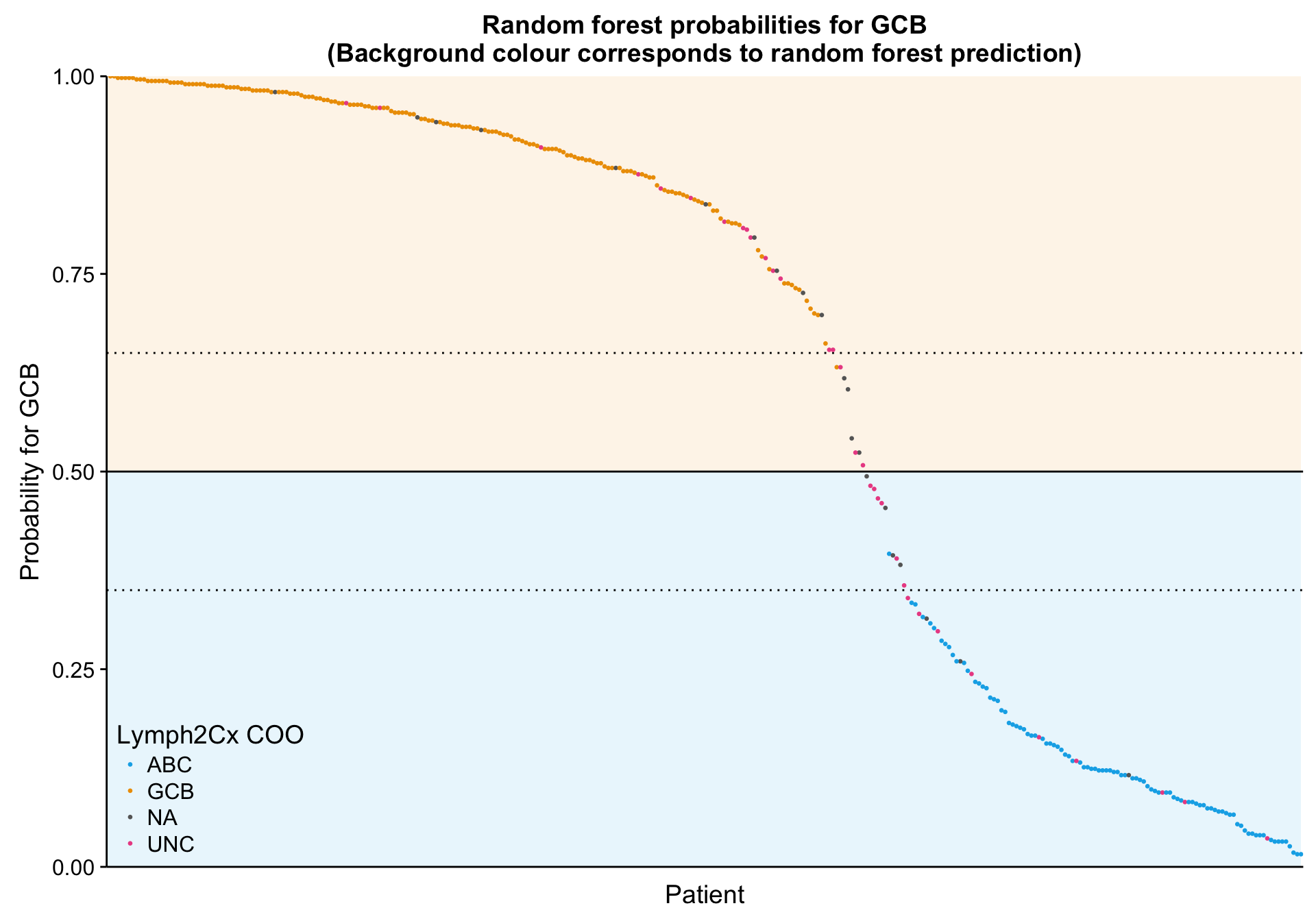
lineplot_mut_rf_prob <-
lineplot_mut_rf_prob_df %>%
ggplot(aes(x = id, y = prob, colour = coo)) +
annotate("rect", xmin = 0, xmax = n_patients, ymin = 0, ymax = 0.5,
fill = colours$coo["ABC"], alpha = 0.1) +
annotate("rect", xmin = 0, xmax = n_patients, ymin = 0.5, ymax = 1,
fill = colours$coo["GCB"], alpha = 0.1) +
geom_hline(yintercept = 0.5) +
geom_hline(yintercept = c(0.35, 0.65), linetype = 3) +
geom_point(aes(colour = coo_ns), size = 0.5) +
scale_color_manual(values = colours$coo) +
place_legend(c(0, 0)) +
scale_x_discrete(labels = NULL) +
scale_y_continuous(limits = c(0, 1), expand = c(0, 0)) +
theme(axis.ticks.x = element_blank()) +
labs(title = paste0("Random forest probabilities for GCB\n",
"(Background colour corresponds to random forest prediction)"),
x = "Patient", y = "Probability for GCB", colour = "Lymph2Cx COO")
lineplot_mut_rf_prob