TreeBuilder3D is an interactive viewer that allows organization of SAGE and other types of gene expression data such as microarrays into hierarchical dendrograms, or phenetic networks (the term 'phenetic' used as the analysis relies on principals, used in phylogenetic analysis by system biology). Might be used as a visual aid when analyzing differences in expression profiles of SAGE libraries, serves as an alternative to Venn diagrams.
Using TreeBuilder3D makes it is possible to load the expression data in the format of plain text files and build a hypothetic tree-like diagram, which describes 'evolutional' relationships between different datasets (such as SAGE libraries). Such diagrams might give one an idea about hierarchical organization of gene expression data, and allow you to associate various expression profiles (represented by SAGE libraries or microarray experiments) with different cellular states or intermediate stages of a decease (such as cancer).
The grouping algorithm of TreeBuilder3D is similar to those used in other clustering method, which generally use Pearson and other metrics to group the similar expression profiles. Unlike them, TreeBuilder3D visualizes not only the grouping but also the relative distances between datasets and presents the knowledge about how 'far' or how 'close' expression profiles are to each other. Besides, as it operates with the data in 3D, it efficiently removes the constrains of 2D space, giving a possibility to view properly scaled distances between datasets.
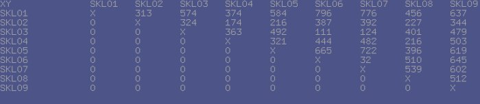
The typical session with TreeBuilder3D consists of two stages: First, the application loads the data and generates the 'distance matrix' - a table containing the distance values for each possible pair of datasets, involved in analysis. These values are generated using different distance metrics and later get normalized for the viewer.
Currently, 5 distance metrics are implemented:
- Quantitative: distance is represented by the ratio of the number of similarly expressed genes to the number of differently expressed genes (statistically filtered by Chi-square test).
- Pearson Squared correlation: distance is a squared Pearson coefficient. Datasets with significantly anticorrelated profiles are considered as 'close'. It is recommended to turn on log scaled mode when using this metric.
- Pearson Uncentered: distance is a squared Pearson coefficient, in which the standard deviation calculated not around mean signal, but around 0 Datasets with significantly anticorrelated profiles are considered as 'close'. It is recommended to turn on log scaled mode when using this metric.
- Euclidean distance: Distance is calculated as a sum of geometric distances between expression values for genes in two sets.
- Manhattan distance: Distance is calculated as sum of absolute differences between expression values for genes in two sets.
Next, the application passes the data to its viewer module, where the phenetic tree is being built. The diagram looks like a set of balls with the labels next to them connected with each other by colored edges. The color of the edge reflects the 'tension' between the nodes, which means the edge is not scaled properly (stretched or compressed).
The brightness of the edge's color shows that the stretching/compression results in gain/loss no less than 50% of original length (dull blue, for stretching and dull red for compression). Or, if the gain/loss of the length for the edge is higher than 50% the color changes to bright blue or bright red. The edge is drawn in black if the stretching/compression changes are within 10% of original size.
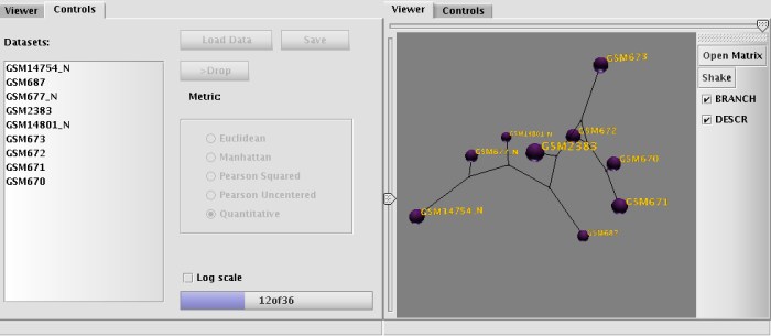
At this point, the user may do a few additional things: It is possible to manipulate the view (Pan, Rotate, Zoom) and it is also possible to regulate the 'density' of the graph with left-side slider and threshold of visibility for the connection (if not in the UPGMA mode). Adjusting visibility (with top-side slider) might help to visualize all or just the shortest connections (which connects the expression profiles which are most similar to each other). BRANCH mode turns on a simple clustering algorithm, which tries to minimize the number of shown connections by leaving visible only the shortest ones. The algorithm is analogous to Neighbor-Joining method for building of hierarchical diagrams. Grouping of nodes starts with connecting the closest libraries first, then the algorithm searches all unclustered libraries against the already grouped ones for the next shortest connection. Gradually, the grouping continues until all libraries are connected.
It is important to note, that positioning of nodes on the graph depends on the original distances, not on the calculations done by NJ algorithm - the later determines only the branching order, while the distances between nodes are shown according to user choice (calculated using Pearson statistics, Euclidean etc.) It is also possible to 'shake' the nodes in the diagram in order to achieve the most relaxed state of the graph.
The application also allows one to save the calculated distance tables into files and later load this tables in viewer module. Adding/Dropping libraries to the analysis set supports multiple selection, so it is possible to load/drop multiple libraries at once.
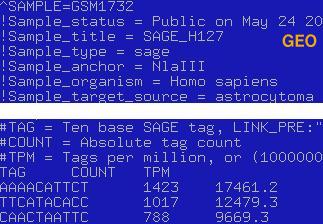
Files with expression data should be formatted in one of two ways: It should be either a list of all tags in a library or tab-delimited list of unique tags with the counts next to them. To allow the analysis of filtered data (cases when a set of tags removed from the list) application supports tag '>TOTAL\t****' which should be placed in the first line of the file (Sample screenshot below). The '>TOTAL' tag allows to normalize libraries properly, otherwise the application sums up all counts for the tags in the file and treat this value as the total number of tags in the library. Tag '>DESCRIPTION' is also supported, and user may pass additional short discription of a dataset, using this tag.
It is also possible to build a diagram using mapped expression data, for example Unigene ids with tag counts associated with them. It will shrink the files considerably and improve the performance of the application.
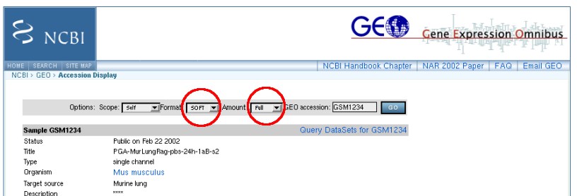
Besides it's own custom file format, the viewer can also read SAGE data available from Gene Expression Omnibus (GEO). In the later case our 3D viewer reads the dataset name and expression information. Prior to comparison of loaded datasets, TreeBuilder performs normalization, using values passed in the header of a file.If the header does not contain the values, needed for normalization, TreeBuilder3D assumes that the data has been normalized. GEO files should be downloaded using the options shown below (parameters should be set to Format:SOFT and Amount:Full).
Current Release
Released Oct 10, 2006, September 16, 2005 release.
Requirements
- Java SDK 1.4 or higher
- Java 3D API (Sun website, not required in case of the package with Java3D included)
- or (for the Java3D part) Java 3D API (Java3D.org website)
Remarks: TreeBuilder3D was designed and tested with Java3D API 1.3.1 under Linux OS. It is a required to have the Java3D API of this particular version, as at the moment 1.3.1 is the newest release available for Linux. We do not provide a version of TreeBuilder3D bundled with Java3D libraries, so the user should install these libraries in order to run the application. No support provided or planned for newer versions of Java3D API (which are available for other platforms). The author does not guarantee taht TreeBuilder3D will run with a version of Java3D API other than 1.3.1